Performance Measures for Multi-Class Problems
For classification problems, classifier performance is typically defined according to the confusion matrix associated with the classifier. Based on the entries of the matrix, it is possible to compute sensitivity (recall), specificity, and precision. For a single cutoff, these quantities lead to balanced accuracy (sensitivity and specificity) or to the F1-score (recall and precision). For evaluate a scoring classifier at multiple cutoffs, these quantities can be used to determine the area under the ROC curve (AUC) or the area under the precision-recall curve (AUCPR).
All of these performance measures are easily obtainable for binary classification problems. Which measure is appropriate depends on the type of classifier. Hard classifiers are non-scoring because they only produce an outcome \(g(x) \in \{1, 2, \ldots, K\}\). Soft classifiers, on the other hand, are scoring classifiers that produce quantities on which a cutoff can be applied in order to find \(g(x)\). For non-scoring classifiers, I introduce two versions of classifier accuracy as well as the micro- and macro-averages of the F1-score. For scoring classifiers, I describe a one-vs-all approach for plotting the precision vs recall curve and a generalization of the AUC for multiple classes.
Data of a non-scoring classifier
To showcase the performance metrics for non-scoring classifiers in the multi-class setting, let us consider a classification problem with \(N = 100\) observations and five classes with \(G = \{1, \ldots, 5\}\):
ref.labels <- c(rep("A", 45), rep("B" , 10), rep("C", 15), rep("D", 25), rep("E", 5))
predictions <- c(rep("A", 35), rep("E", 5), rep("D", 5),
                 rep("B", 9), rep("D", 1),
                 rep("C", 7), rep("B", 5), rep("C", 3),
                 rep("D", 23), rep("C", 2),
                 rep("E", 1), rep("A", 2), rep("B", 2))
df <- data.frame("Prediction" = predictions, "Reference" = ref.labels, stringsAsFactors=TRUE)
Accuracy and weighted accuracy
Conventionally, multi-class accuracy is defined as the average number of correct predictions:
\[\text{accuracy} = \frac{1}{N} \sum_{k=1}^{|G|} \sum_{x: g(x) = k} I \left(g(x) = \hat{g}(x)\right)\]
where \(I\) is the indicator function, which returns 1 if the classes match and 0 otherwise.
To be more sensitive to the performance for individual classes, we can assign a weight \(w_k\) to every class such that \(\sum_{k=1}^{|G|} w_k = 1\). The higher the value of \(w_k\) for an individual class, the greater is the influence of observations from that class on the weighted accuracy. The weighted accuracy is determined by:
\[\text{weighted accuracy} = \sum_{k=1}^{|G|} w_i \sum_{x: g(x) = k} I\left(g(x) = \hat{g}(x)\right)\,.\]
To weight all classes equally, we can set \(w_k = \frac{1}{|G|}\,,\forall k \in \{1, \ldots, G\}\). Note that when anything other than uniform weights are used, it is hard to find a rational argument for a certain combination of weights.
Calculating accuracy and weighted accuracy
The accuracy is very easy to calculate:
calculate.accuracy <- function(predictions, ref.labels) {
    return(length(which(predictions == ref.labels)) / length(ref.labels))
}
calculate.w.accuracy <- function(predictions, ref.labels, weights) {
    lvls <- levels(ref.labels)
    if (length(weights) != length(lvls)) {
        stop("Number of weights should agree with the number of classes.")
    }
    if (sum(weights) != 1) {
        stop("Weights do not sum to 1")
    }
    accs <- lapply(lvls, function(x) {
        idx <- which(ref.labels == x)
        return(calculate.accuracy(predictions[idx], ref.labels[idx]))
    })
    acc <- mean(unlist(accs))
    return(acc)
}
acc <- calculate.accuracy(df$Prediction, df$Reference)
print(paste0("Accuracy is: ", round(acc, 2)))
## [1] "Accuracy is: 0.78"weights <- rep(1 / length(levels(df$Reference)), length(levels(df$Reference)))
w.acc <- calculate.w.accuracy(df$Prediction, df$Reference, weights)
print(paste0("Weighted accuracy is: ", round(w.acc, 2)))## [1] "Weighted accuracy is: 0.69"Note that the weighted accuracy with uniform weights is lower (0.69) than the overall accuracy (0.78) because it gives equal contribution to the predictive performance for the five classes, independent of their number of observations.
Micro and macro averages of the F1-score
Micro and macro averages represent two ways of interpreting confusion matrices in multi-class settings. Here, we need to compute a confusion matrix for every class \(g_i \in G = \{1, \ldots, K\}\) such that the \(i\)-th confusion matrix considers class \(g_i\) as the positive class and all other classes \(g_j\) with \(j \neq i\) as the negative class. Since each confusion matrix pools all observations labeled with a class other than \(g_i\) as the negative class, this approach leads to an increase in the number of true negatives, especially if there are many classes.
To exemplify why the increase in true negatives is problematic, imagine there are 10 classes with 10 observations each. Then the confusion matrix for one of the classes may have the following structure:
| Prediction/Reference | Class 1 | Other Class |
|---|---|---|
| Class 1 | 8 | 10 |
| Other Class | 2 | 80 |
Based on this matrix, the specificity would be \(\frac{80}{80 + 10} = 88.9\%\) although class 1 was only correctly predicted in 8 out of 18 instances (precision 44.4%). Thus, since the negative class is predominant, the specificity becomes inflated. Thus, micro- and macro averages are only defined for the F1-score and not for the balanced accuracy, which relies on the true negative rate.
In the following we will use \(TP_i\), \(FP_i\), and \(FN_i\) to respectively indicate true positives, false positives, and false negatives in the confusion matrix associated with the \(i\)-th class. Moreover, let precision be indicated by \(P\) and recall by \(R\).
The micro average
The micro average has its name from the fact that it pools the performance over the smallest possible unit (i.e. over all samples):
\[ \begin{align*} P_{\rm{micro}} &= \frac{\sum_{i=1}^{|G|} TP_i}{\sum_{i=1}^{|G|} TP_i+FP_i} \\ R_{\rm{micro}} &= \frac{\sum_{i=1}^{|G|} TP_i}{\sum_{i=1}^{|G|} TP_i + FN_i} \end{align*} \]
The micro-averaged precision, \(P_{\rm{micro}}\), and recall, \(R_{\rm{micro}}\), give rise to the micro F1-score:
\[F1_{\rm{micro}} = 2 \frac{P_{\rm{micro}} \cdot R_{\rm{micro}}}{P_{\rm{micro}} + R_{\rm{micro}}}\]
If a classifier obtains a large \(F1_{\rm{micro}}\), this indicates that it performs well overall. The micro-average is not sensitive to the predictive performance for individual classes. As a consequence, the micro-average can be particularly misleading when the class distribution is imbalanced.
The macro average
The macro average has its name from the fact that it averages over larger groups, namely over the performance for individual classes rather than observations:
\[ \begin{align*} P_{\rm{macro}} &= \frac{1}{|G|} \sum_{i=1}^{|G|} \frac{TP_i}{TP_i+FP_i} = \frac{\sum_{i=1}^{|G|} P_i}{|G|}\\ R_{\rm{macro}} &= \frac{1}{|G|} \sum_{i=1}^{|G|} \frac{TP_i}{TP_i + FN_i} = \frac{\sum_{i=1}^{|G|} R_i}{|G|} \end{align*} \]
The macro-averaged precision and recall give rise to the macro F1-score:
\[F1_{\rm{macro}} = 2 \frac{P_{\rm{macro}} \cdot R_{\rm{macro}}}{P_{\rm{macro}} + R_{\rm{macro}}}\]
If \(F1_{\rm{macro}}\) has a large value, this indicates that a classifier performs well for each individual class. The macro-average is therefore more suitable for data with an imbalanced class distribution.
Computing micro- and macro averages in R
Here, I demonstrate how the micro- and macro averages of the F1-score can be computed in R.
One-vs-all confusion matrices
The first step for finding micro- and macro averages involves computing one-vs-all confusion matrices for each class. We will use the confusionMatrix function from the caret package to determine the confusion matrices:
library(caret) # for confusionMatrix function
cm <- vector("list", length(levels(df$Reference)))
for (i in seq_along(cm)) {
    positive.class <- levels(df$Reference)[i]
    # in the i-th iteration, use the i-th class as the positive class
    cm[[i]] <- confusionMatrix(df$Prediction, df$Reference,
                               positive = positive.class)
}
Now that all class-specific confusion matrices are stored in cm, we can summarize the performance across all classes:
metrics <- c("Precision", "Recall")
print(cm[[1]]$byClass[, metrics])
## Precision Recall
## Class: A 0.9459459 0.7777778
## Class: B 0.5625000 0.9000000
## Class: C 0.8333333 0.6666667
## Class: D 0.7931034 0.9200000
## Class: E 0.1666667 0.2000000These data indicate that, overall, performance is quite high. However, our hypothetical classifier underperforms for individual classes such as class B (precision) and class E (both precision and recall). We will now investigate how micro- and macro-averages of the F1-score are influenced by the predictions of the model.
Overall performance with micro-averaged F1
To determine \(F1_{\rm{micro}}\), we need to determine \(TP_i\), \(FP_i\), and \(FN_i\) \(\forall i \in \{1, \ldots, K\}\). This is done by the get.conf.stats function. The function get.micro.f1 then simply aggregates the counts and calculates the F1-score as defined above.
get.conf.stats <- function(cm) {
    out <- vector("list", length(cm))
    for (i in seq_along(cm)) {
        x <- cm[[i]]
        tp <- x$table[x$positive, x$positive]
        fp <- sum(x$table[x$positive, colnames(x$table) != x$positive])
        fn <- sum(x$table[colnames(x$table) != x$positie, x$positive])
        # TNs are not well-defined for one-vs-all approach
        elem <- c(tp = tp, fp = fp, fn = fn)
        out[[i]] <- elem
    }
    df <- do.call(rbind, out)
    rownames(df) <- unlist(lapply(cm, function(x) x$positive))
    return(as.data.frame(df))
}
get.micro.f1 <- function(cm) {
    cm.summary <- get.conf.stats(cm)
    tp <- sum(cm.summary$tp)
    fn <- sum(cm.summary$fn)
    fp <- sum(cm.summary$fp)
    pr <- tp / (tp + fp)
    re <- tp / (tp + fn)
    f1 <- 2 * ((pr * re) / (pr + re))
    return(f1)
}
micro.f1 <- get.micro.f1(cm)
print(paste0("Micro F1 is: ", round(micro.f1, 2)))
## [1] "Micro F1 is: 0.88"With a value of 0.88, \(F_1{\rm{micro}}\) is quite high, which indicates a good overall performance. As expected, the micro-averaged F1, did not really consider that the classifier had a poor performance for class E because there are only 5 measurements in this class that influence \(F_1{\rm{micro}}\).
Class-specific performance with macro-averaged F1
Since each confusion matrix in cm already stores the one-vs-all prediction performance, we just need to extract these values from one of the matrices and calculate \(F1_{\rm{macro}}\) as defined above:
get.macro.f1 <- function(cm) {
    c <- cm[[1]]$byClass # a single matrix is sufficient
    re <- sum(c[, "Recall"]) / nrow(c)
    pr <- sum(c[, "Precision"]) / nrow(c)
    f1 <- 2 * ((re * pr) / (re + pr))
    return(f1)
}
macro.f1 <- get.macro.f1(cm)
print(paste0("Macro F1 is: ", round(macro.f1, 2)))
## [1] "Macro F1 is: 0.68"With a value of 0.68, \(F_{\rm{macro}}\) is decidedly smaller than the micro-averaged F1 (0.88). Since the classifier for class E performs poorly (precision: 16.7%, recall: 20%) and contributes \(\frac{1}{5}\) to \(F_{\rm{macro}}\), it is lower than \(F1_{\rm{micro}}\).
Note that, for the present data set, micro- and macro-averaged F1 have a similar relationship to each other as the overall (0.78) and weighted accuracy (0.69).
Precision-recall curves and AUC
The area under the ROC curve (AUC) is a useful tool for evaluating the quality of class separation for soft classifiers. In the multi-class setting, we can visualize the performance of multi-class models according to their one-vs-all precision-recall curves. The AUC can also be generalized to the multi-class setting.
One-vs-all precision-recall curves
As discussed in this Stack Exchange thread, we can visualize the performance of a multi-class model by plotting the performance of \(K\) binary classifiers.
This approach is based on fitting \(K\) one-vs-all classifiers where in the \(i\)-th iteration, group \(g_i\) is set as the positive class, while all classes \(g_j\) with \(j \neq i\) are considered to be the negative class. Note that this method should not be used to plot conventional ROC curves (TPR vs FPR) since the FPR will be underestimated due to the large number of negative examples resulting from the dichotimization. Instead, precision and recall should be considered:
library(ROCR) # for ROC curves
library(klaR) # for NaiveBayes
data(iris) # Species variable gives the classes
response <- iris$Species
set.seed(12345)
train.idx <- sample(seq_len(nrow(iris)), 0.6 * nrow(iris))
iris.train <- iris[train.idx, ]
iris.test <- iris[-train.idx, ]
plot(x=NA, y=NA, xlim=c(0,1), ylim=c(0,1),
     ylab="Precision",
     xlab="Recall",
     bty='n')
colors <- c("red", "blue", "green")
aucs <- rep(NA, length(levels(response))) # store AUCs
for (i in seq_along(levels(response))) {
  cur.class <- levels(response)[i]
  binary.labels <- as.factor(iris.train$Species == cur.class)
  # binarize the classifier you are using (NB is arbitrary)
  model <- NaiveBayes(binary.labels ~ ., data = iris.train[, -5])
  pred <- predict(model, iris.test[,-5], type='raw')
  score <- pred$posterior[, 'TRUE'] # posterior for  positive class
  test.labels <- iris.test$Species == cur.class
  pred <- prediction(score, test.labels)
  perf <- performance(pred, "prec", "rec")
  roc.x <- unlist(perf@x.values)
  roc.y <- unlist(perf@y.values)
  lines(roc.y ~ roc.x, col = colors[i], lwd = 2)
  # store AUC
  auc <- performance(pred, "auc")
  auc <- unlist(slot(auc, "y.values"))
  aucs[i] <- auc
}
lines(x=c(0,1), c(0,1))
legend("bottomright", levels(response), lty=1,
    bty="n", col = colors)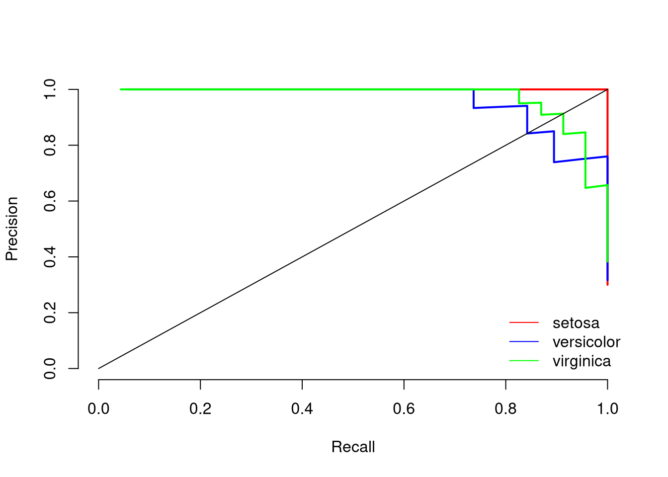
print(paste0("Mean AUC under the precision-recall curve is: ", round(mean(aucs), 2)))## [1] "Mean AUC under the precision-recall curve is: 0.99"The plot indicates that setosa can be predicted very well, while versicolor and virginica are harder to predict. The mean AUC of 0.99 indicates that the model separates the three classes very well.
Generalizations of the AUC for the multi-class setting
There are several generalizations of the AUC for the multi-class setting. Here, I will focus on the generalization established by Hand and Till in 2001.
Generalized AUC for a single decision value
The multiclass.roc function from the pROC package can be used to determine the AUC when a single quantity allows for the separation of the classes. In contrast to the documentation of the function, the function does not seem to implement the approach from Hand and Till
because the class predictions are not considered. However, the documentation warns about this function being in beta phase. I am currently waiting for a response from the package authors about the multiclass.roc function to verify whether my understanding is correct.
library(pROC)
data(aSAH)
auc <- multiclass.roc(aSAH$gos6, aSAH$s100b)
print(auc$auc)
## Multi-class area under the curve: 0.654The calculated AUC of the function is simply the mean AUC from all pairwise class comparisons.
Generalization of the AUC by Hand and Till
The following describes the generalization of the AUC from Hand and Till, 2001.
Assume that the classes are labeled as \(0, 1, 2, \ldots, c - 1\) with \(c > 2\). To generalize the AUC, we consider pairs of classes \((i,j)\). A good classifier should assign a high probability to the correct class, while assigning low probabilities to the other classes. This can be formalized in the following way.
Let \(\hat{A}(i|j)\) indicate the probability that a randomly drawn member of class \(j\) has a lower probability for class \(i\) than a randomly drawn member of class \(i\). Let \(\hat{A}(j|i)\) be defined correspondingly. We can calculate \(\hat{A}(i|j)\) using the following definitions:
- \(\hat{p}(x_l)\) is the estimated probability that observation \(x_l\) originates from class \(i\).
- For all class \(i\) observations \(x_l\), let \(f_l = \hat{p}(x_l)\) be the estimated probability of belonging to class \(i\).
- For all class \(j\) observations \(x_l\), let \(g_l = \hat{p}(x_l)\) be the estimated probability of belonging to class \(i\).
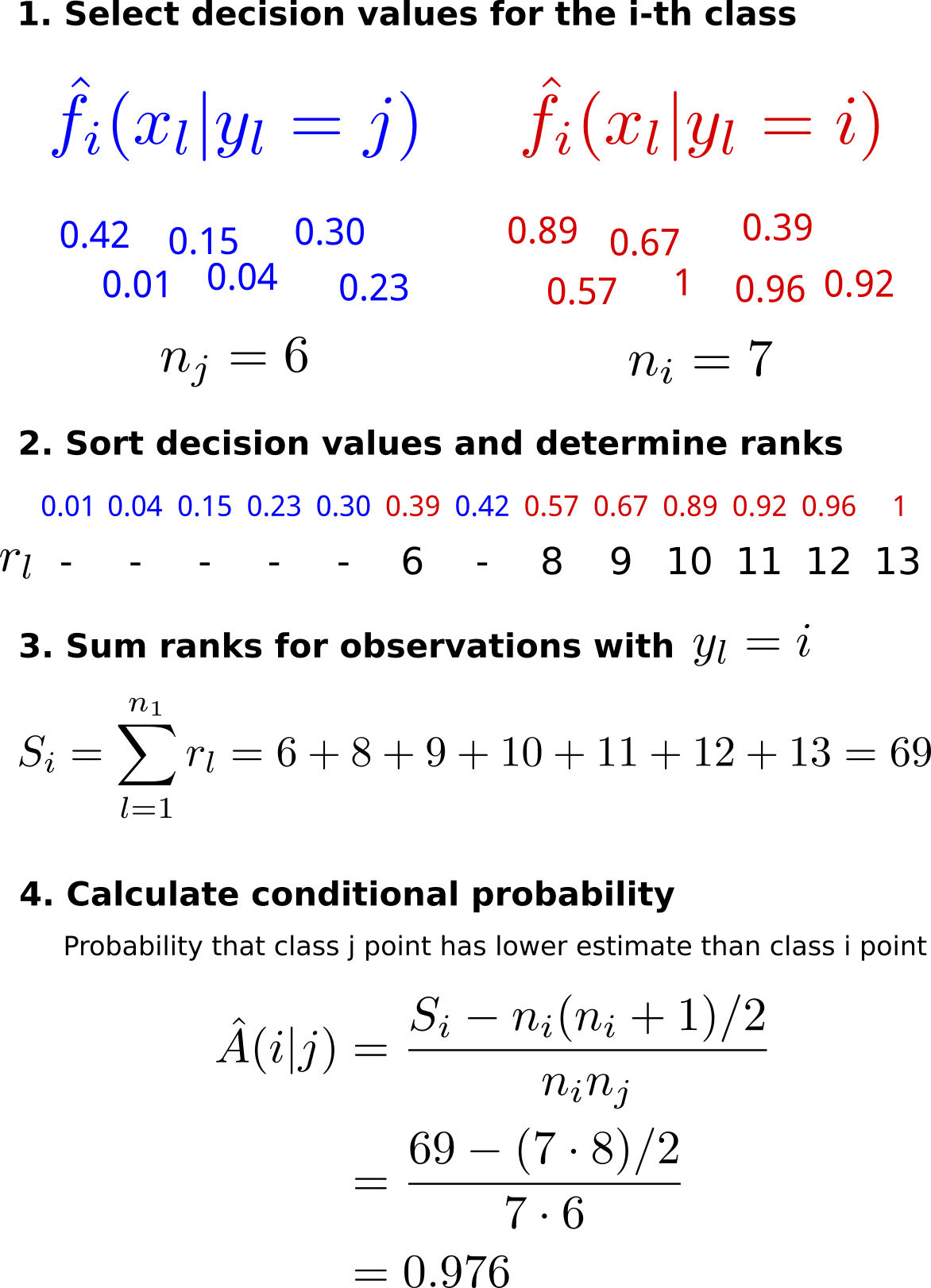
Now, we rank the combined set of values \(\{g_1, \ldots, g_{n_j}, f_1, \ldots, f_{n_i}\}\) in increasing order. Let \(r_l\) be the rank of the \(l\)-th observation from class \(i\). Then, the total number of pairs of points in which the class \(j\) point has a smaller estimated probability of belonging to class \(i\) than the class \(i\) point is given by
\[\sum_{l=1}^{n_i} r_l - l = \sum_{l=1}^{n_i} r_l - \sum_{l=1}^{n_i} l = S_i - n_i(n_i +1)/2 \]
where \(S_i\) is the sum of the ranks from the class \(i\) samples. Because there are \(n_0 n_1\) pairs of points from two classes, the probability that a randomly chosen class \(j\) point has a lower estimated probability of belonging to class \(i\) than a randomly chosen class \(i\) point is:
\[\hat{A}(i|j) = \frac{S_i - n_i(n_i +1)/2}{n_i n_j}\,. \]
Since we cannot distinguish \(\hat{A}(i|j)\) from \(\hat{A}(j|i)\), we define
\[\hat{A}(i,j) = \frac{1}{2} \left(\hat{A}(i|j) + \hat{A}(j|i)\right)\]
as the measure for the separability for classes \(i\) and \(j\). The overall AUC of a multi-class classifier is then given by the average value for \(\hat{A}(i,j)\):
\[ M = \frac{2}{c(c-1)} \sum_{i < j} \hat{A}(i,j) \]
Here, the multiplier is \(\frac{2}{c (c-1)}\) because there are \(c (c-1)\) ways in which distinct pairs can be constructed taking different orderings into account. Since only half of these pairs are computed, the enumerator has a value of 2.
Example for computing conditional probabilities
Please condider the following diagram for an example of how the conditional probabilties are computed.
Implementation of the AUC generalization from Hand and Till
It seems that there is no publicly available implementation of the multi-class generalization of the AUC due to Hand and Till (2001). Thus, I wrote an implementation. The function compute.A.conditional determines \(\hat{A}(i|j)\). The multiclass.auc function computes \(\hat{A}(i,j)\) for all pairs of classes with \(i < j\) and then calculates the mean of the resulting values. The output is the generalized AUC, \(M\), and the attribute pair_AUCs indicates the values for \(A(i,j)\).
compute.A.conditional <- function(pred.matrix, i, j, ref.outcome) {
    # computes A(i|j), the probability that a randomly
    # chosen member of class j has a lower estimated probability (or score)
    # of belonging to class i than a randomly chosen member of class i

    # select predictions of class members
    i.idx <- which(ref.outcome == i)
    j.idx <- which(ref.outcome == j)
    pred.i <- pred.matrix[i.idx, i] # p(G = i) assigned to class i observations
    pred.j <- pred.matrix[j.idx, i] # p(G = i) assigned to class j observations
    all.preds <- c(pred.i, pred.j)
    classes <- c(rep(i, length(pred.i)), rep(j, length(pred.j)))
    o <- order(all.preds)
    classes.o <- classes[o]
    # Si: sum of ranks from class i observations
    Si <- sum(which(classes.o == i))
    ni <- length(i.idx)
    nj <- length(j.idx)
    # calculate A(i|j)
    A <- (Si - ((ni * (ni + 1))/2)) / (ni * nj)
    return(A)
}

multiclass.auc <- function(pred.matrix, ref.outcome) {
    labels <- colnames(pred.matrix)
    A.ij.cond <- utils::combn(labels, 2, function(x, pred.matrix, ref.outcome) {x
        i <- x[1]
        j <- x[2]
        A.ij <- compute.A.conditional(pred.matrix, i, j, ref.outcome)
        A.ji <- compute.A.conditional(pred.matrix, j, i, ref.outcome)
        pair <- paste0(i, "/", j)
        return(c(A.ij, A.ji))
    }, simplify = FALSE, pred.matrix = pred.matrix, ref.outcome = ref.outcome)
    c <- length(labels)
    pairs <- unlist(lapply(combn(labels, 2, simplify = FALSE), function(x) paste(x, collapse = "/")))
    A.mean <- unlist(lapply(A.ij.cond, mean))
    names(A.mean) <- pairs
    A.ij.joint <- sum(unlist(A.mean))
    M <- 2 / (c * (c-1)) * A.ij.joint
    attr(M, "pair_AUCs") <- A.mean
    return(M)
}
model <- NaiveBayes(iris.train$Species ~ ., data = iris.train[, -5])
pred <- predict(model, iris.test[,-5], type='raw')
pred.matrix <- pred$posterior
ref.outcome <- iris.test$Species
M <- multiclass.auc(pred.matrix, ref.outcome)
print(paste0("Generalized AUC is: ", round(as.numeric(M), 3)))
## [1] "Generalized AUC is: 0.991"print(attr(M, "pair_AUCs")) # pairwise AUCs## setosa/versicolor setosa/virginica versicolor/virginica
## 1.00000 1.00000 0.97254Using this approach, the generalized AUC is 0.988, which is surprisingly similar to the mean value from the precision-recall curves of the binary one-vs-all classifiers. The interpretation of the resulting pairwise AUCs is also similar. While the AUCs for separating setosa/versicolor and setosa/virginica are both 1, the AUC for versicolor/virginica is slightly smaller, which is in line with our previous finding that observations from versicolor and virginica are harder to predict accurately.
Other ROC-based approaches
There are also other ROC-based approaches available. For brevity’s sake, I will, however, not discuss them here at the moment.
Summary
For multi-class problems, similar measures as for binary classification are available.
- For hard classifiers, you can use the (weighted) accuracy as well as micro or macro-averaged F1 score.
- For soft classifiers, you can determine one-vs-all precision-recall curves or use the generalization of the AUC from Hand and Till.


Comments
Krish S
16 Apr 20 22:54 UTC
Matthias Döring
17 Apr 20 16:01 UTC
Your welcome!
Regarding the approach from Hand and Till: The functionality for Hand and Till should now be available from the pROC package via multiclass.roc, at least it’s in the GitHub master at: https://github.com/xrobin/pROC
Why is their approach better than taking the mean? Well, it’s all about interpretability. If you take the mean you do not take information about the classes into account. Hand and Till, however, considers how far apart the class predictions are, which gives you a more informative value.
Krish S
21 Apr 20 23:39 UTC
Carsten
24 Apr 20 14:39 UTC
But I might be wrong but are you sure that you haven’t switched the explanations for macro/micro average F1 Scores? Because micro avg F1 is preferable if you suspect there is a class imbalance. Please let me know what you think.
Pablo
19 May 20 00:33 UTC
Matthias
19 May 20 06:33 UTC
Huanfa Chen
15 Jul 20 17:43 UTC
Matthias
15 Jul 20 20:19 UTC
Dear Huanfa, Let’s assume we have:
Then we can define the measures as
So, as you can see, in general, the unweighted accuracy is not the same as the micro-average precision/recall. However, they could be the same under special circumstances. For example, for TN = FN = 0, unweighted accuracy and micro-average precision would be identical.