Inference vs Prediction
Generative modeling or predictive modeling?
The terms inference and prediction both describe tasks where we learn from data in a supervised manner in order to find a model that describes the relationship between the independent variables and the outcome. Inference and prediction, however, diverge when it comes to the use of the resulting model:
- Inference: Use the model to learn about the data generation process.
- Prediction: Use the model to predict the outcomes for new data points.
Since inference and prediction pursue contrasting goals, specific types of models are associated with the two tasks.
Model interpretability is a necessity for inference
In essence, the difference between models that are suitable for inference and those that are not boils down to model interpretability. What do I mean with model interpretability? I consider a model interpretable if a human, particularly a layman, could retrace how the model generates its estimates. Consider the following approaches for prediction:
- Interpretable: Generalized linear models (e.g. linear regression, logistic regression), linear discriminant analysis, linear support vector machines (SVMs), decision trees
- Less interpretable: neural networks, non-linear SVMs, random forests
Only a subset of interpretable methods is useful for inference. For example, linear SVMs are interpretable because they provide a coefficient for every feature such that it is possible to explain the impact of individual features on the prediction. However, SVMs do not allow for estimating the uncertainty associated with the model coefficients (e.g. the variance) and it is not possible to obtain an implicit measure of model confidence. Note that SVMs are capable of outputting probabilities but these probabilities are just a transformation of the decision values and are not basted on the confidence associated with the parameter estimates. This is why even interpretable methods such as linear SVMs and decision trees are unsuitable for inference.
In contrast, consider linear regression, which assumes that the data follow a Gaussian distribution. These models determine the standard error of the coefficient estimates and output confidence intervals. Since linear regression allows us to understand the probabilistic nature of the data generation process, it is a suitable method for inference. Bayesian methods are particularly popular for inference because these models can be adjusted to incorporate various assumptions about the data generation process.
Examples for prediction and inference
Merely using a model that is suitable for inference does not mean that you are actually performing inference. What matter is how you are using the model. For example, although generalized linear models are suitable for inference, I recently used them solely for prediction purposes. Consider the following examples that make the distinction between prediction and inference clearer:
- Prediction: You want to predict future ozone levels using historic data. Since you believe that there is a linear relationship between the ozone level and measurements of temperature, solar radiation, and wind, you fit several linear models (e.g. using different sets of features) on the training data and select the model minimizing the loss on the test set. Finally, you use the selected model for predicting the ozone level. Note that you do not care at all about the Gaussian assumption of the model or the additional information that is available on the model estimates as long as the model minimizes the test error.
- Inference: You want to understand how ozone levels are influenced by temperature, solar radiation, and wind. Since you assume that the residuals are normally distributed, you use a linear regression model. In order to harness the information from the full data set and you do not care about predictive accuracy, you fit the model on the full data set. On the basis of the fitted model, you interpret the role of the features on the measured ozone level, for example, by considering the confidence bands of the estimates.
Workflows for inference and prediction
The basic workflows for inference and prediction are described in the following sections.
Inference
- Modeling: Reason about the data generation process and choose the stochastic model that approximates the data generation process best.
- Model validation: Evaluate the validity of the stochastic model using residual analysis or goodness-of-fit tests.
- Inference: Use the stochastic model to understand the data generation process .
Prediction
- Modeling: Consider several different models and different parameter settings.
- Model selection: Identify the model with the greatest predictive performance using validation/test sets; select the model with the highest performance on the test set.
- Prediction: Apply the selected model on new data with the expectation that the selected model also generalizes to the unseen data.
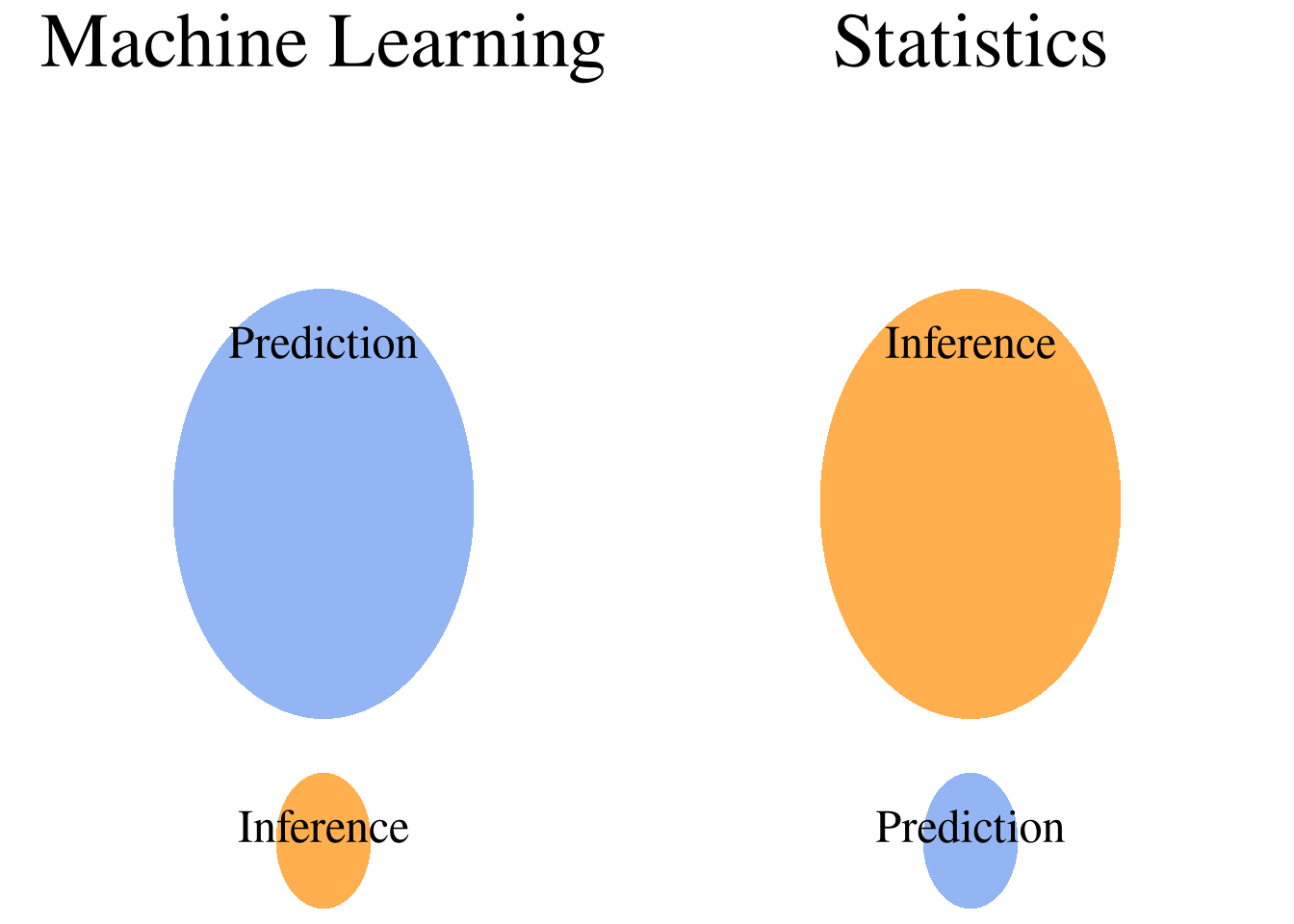
The two modeling communities
Note that machine learning is often concerned with predictive modeling, while the statistical community often relies on stochastic models that perform inference. Due to the complexity of machine learning models, they are often treated as black boxes. For inference problems, on the other hand, the working principles of used models are well understood.
Three contradictions in statistical modeling
In his famous 2001 paper, Leo Breiman argued that there are three revolutions in the modeling community, which are represented by the following terms:
- Rashomon: There is often not a single model that fits a data set best but there usually is a multiplicity of models that are similarly appropriate. The term Rashomon refers to a classic 1950 Japanese feature film in which various characters depict different and even contradictory versions of the same incident.
- Occam: The simplest model is often the most interpretable. However, the simplest model is also often not the the most accurate model for a given task. Occam refers to William of Occam’s razor, which states that Entities should not be multiplied beyond necessity, underlining the importance of simplicity.
- Bellman: Large feature spaces are often seen as a disadvantage. However, modern machine learning methods heavily rely on expanding the feature space in order to improve predictive accuracy. So, are we subject to a curse or a blessing of dimensionality? The term curse of dimensionality was coined by Richard Bellman. The term is used to emphasize the challenges of statistical modeling in large feature spaces.
Blessing or curse of dimensionality?
Predictive modeling particularly embraces the idea that high dimensionality is a blessing. All of the recently developed popular machine learning models such as neural networks and SVMs rely on the idea of expanding the feature space in order to learn about the non-linear relationships between the independent variables. As a consequence, these models can also be thought to violate Occam’s razor because these models do not utilize compact representations of the variables but rely on partially redundant encodings.
Generative modeling, on the other hand, is often concerned with feature elimination in order to allow for improved interpretability and generalizability. Since these methods strive for simple models for explaining the data generation process with few features, they simultaneously fulfill Occam’s razor and circumvent the curse of dimensionality.
Feature selection and Rashomon
Models based on feature selection are, however, much more affected by Rashomon, the multiplicity of appropriate models. Imagine you are doing generative modeling and the original data set contains 10,000 features. Using a notion of variable importance, you reduce the number of features down to 100. You then interpret the resulting model according to the 100 features. Now, the question is: Is this model the only way to view the data generation process?
Probably not because, stochastically, it is likely that there exists another model with a different set of 100 features that explains the outcome similarly well. This is due to the existence of a huge number of subsets with exactly 1000 features, namely \({100\,000 \choose 100} = 10^{2430}\). Thus, when performing feature selection, small perturbations in the data may lead to the selection of a model using a different feature subset.
Summary
Prediction and inference can be differentiated according to the following criteria:
| Criterion | Prediction | Inference |
|---|---|---|
| Model Selection | - Evaluate a variety of models - Select the best-performing model |
- Reason about the data generation process - Select model whose assumptions seem most reasonable |
| Validation | - Empirically determine loss on test set | - Use goodneess-of-fit tests |
| Application | - Predict the outcome for new samples | - Use the model to explain the data generation process |
| Ramnifcations | - Model interpretability suffers - Model validity shown for the test set - Model may overfit if the test data are similar to the training data |
- High model interpretability - Model validity is uncertain since predictive accuracy was not considered - Overfitting prevented through simplified assumptions |
Outlook
So what can the communities of predictive and generative modeling learn from each other? In my opinion, practitioners of machine learning should spend more time with the data in order to make well-informed decisions about the type of predictive model that is used. In many prediction scenarios, well-established methods such as SVMs or neural networks are used without thinking about the alternatives according to the saying if all you have is a hammer, everything looks like a nail. However, there may be other models that may be more appropriate to a given data set, for example because they perform better, allow for improved generalizability, or because they are more interpretable.
Additionally, there should be more skepticism about the dogmatic use of the test error as the sole measure of model validity. Particularly in settings where the test set is similar to the training data, a low test error may not guarantee a low generalization error. Finally, further effort should be made in order to peel away some of the layers of dark color that render predictive models intransparent.
In the inference setting, model performance should be included as a criterion for the evaluation of model validity since it is hazardous to draw conclusions from an inaccurate model. If the validity of a model has not been sufficiently established, all interpretations should be taken with a grain of salt and it may be worth to investigate the perspectives that other models offer. Additionally, model assumptions should be well argumented rather than assuming a certain distribution (e.g. normal) for mere convenience.
Finally, when pruning the feature space (in both inference and prediction), one should judiciously decide on the feature selection criterion and be aware that the selected model may not be the only reasonable model for the data at hand. To demonstrate the validity of the selected features, resampling methods such as the bootstrap can be used to demonstrate the robustness of the selected variables.


Comments
Nupur
12 Feb 20 18:16 UTC
Ashar
14 Jun 20 12:39 UTC
Lastika Sethi
11 Jul 20 13:22 UTC
Oliver Faust
17 Oct 20 06:53 UTC