Linear prediction models assume that there is a linear relationship between the independent variables and the dependent variable. Therefore, these models exhibit high bias and low variance.
The high bias of these models is due to the assumption of nonlinearity. If this assumption does not sufficiently represent the data, then linear models will be inaccurate.
On the other hand, linear models also have a low variance. This means that if several linear models would be trained using different data, they would perform similarly on the same test data set. This is because linear models are inflexible because there are few parameters to be tuned.
Thus, linear models are interpretable and robust. However, if their assumptions are not met, they willl perform poorly.
When do use linear models?
Linear models excel under the following circumstances:
There are few data available, which would lead to overfitting with more complex models.
There are indications for a linear association between features and outcome.
Interpretation rather than predictive performance alone is important.
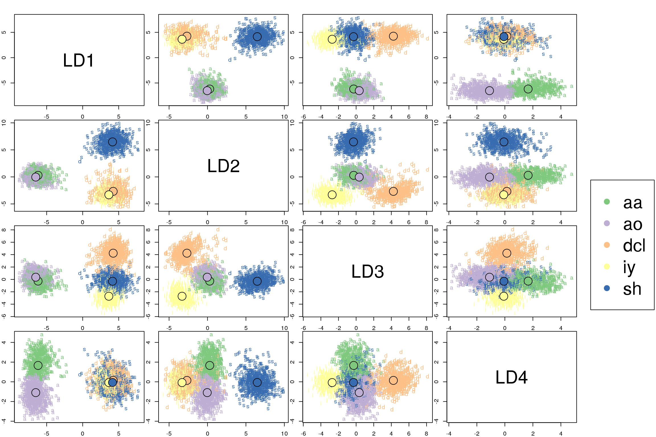
Discriminant analysis encompasses methods that can be used for both classification and dimensionality reduction. Linear discriminant analysis (LDA) is particularly popular because it is both a classifier and a dimensionality reduction technique. Quadratic discriminant analysis (QDA) is a variant of LDA that allows for non-linear separation of data. Finally, regularized discriminant analysis (RDA) is a compromise between LDA and QDA.
This post focuses mostly on LDA and explores its use as a classification and visualization technique, both in theory and in practice.
Interpreting generalized linear models (GLM) obtained through glm is similar to interpreting conventional linear models. Here, we will discuss the differences that need to be considered.
Basics of GLMs GLMs enable the use of linear models in cases where the response variable has an error distribution that is non-normal. Each distribution is associated with a specific canonical link function. A link function \(g(x)\) fulfills \(X \beta = g(\mu)\). For example, for a Poisson distribution, the canonical link function is \(g(\mu) = \text{ln}(\mu)\).
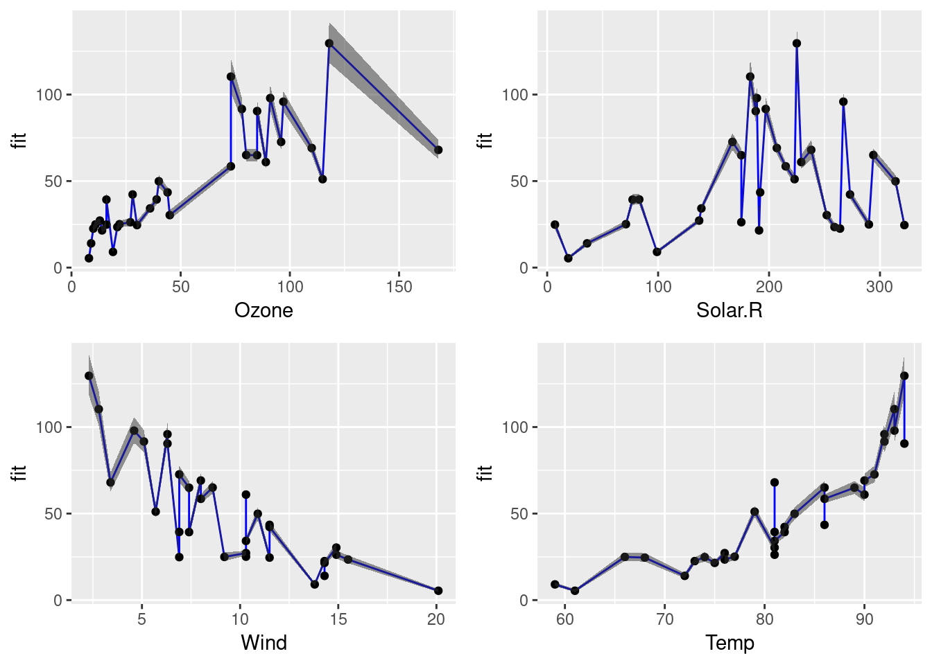
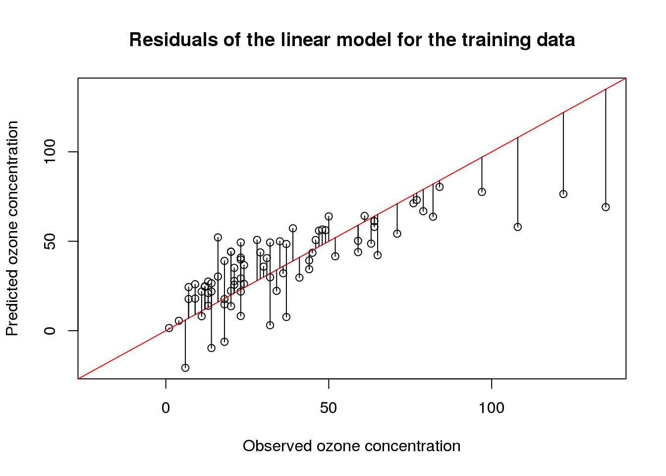
In a previous post, I have introduced the airquality data set in order to demonstrate how linear models are interpreted. In this post, I will start with a basic linear model and, from there, try to find a linear model with a better fit.
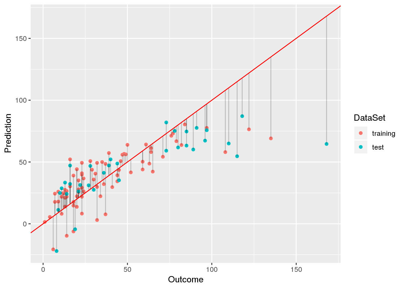
Data preprocessing Since the airquality data set contains some missing values, we will remove those before we begin to fit models and select 70% of the samples for training and use the remainder for testing:
Although linear models are one of the simplest machine learning techniques, they are still a powerful tool for predictions. This is particularly due to the fact that linear models are especially easy to interpret. Here, I discuss the most important aspects when interpreting linear models by example of ordinary least-squares regression using the airquality data set.
The airquality data set The airquality data set contains 154 measurements of the following four air quality metrics as obtained in New York: