Finding a Suitable Linear Model for Ozone Prediction
In a previous post, I have introduced the airquality data set in order to demonstrate how linear models are interpreted. In this post, I will start with a basic linear model and, from there, try to find a linear model with a better fit.
Data preprocessing
Since the airquality data set contains some missing values, we will remove those before we begin to fit models and select 70% of the samples for training and use the remainder for testing:
data(airquality)
ozone <- subset(na.omit(airquality),
        select = c("Ozone", "Solar.R", "Wind", "Temp"))
set.seed(123)
N.train <- ceiling(0.7 * nrow(ozone))
N.test <- nrow(ozone) - N.train
trainset <- sample(seq_len(nrow(ozone)), N.train)
testset <- setdiff(seq_len(nrow(ozone)), trainset)
Ordinary least-squares model
As a baseline model, we will use an ordinary least-squares (OLS) model. Before defining the model, we define a function for plotting linear models:
rsquared <- function(test.preds, test.labels) {
    return(round(cor(test.preds, test.labels)^2, 3))
}
plot.linear.model <- function(model, test.preds = NULL, test.labels = NULL,
                            test.only = FALSE) {
    # ensure that model is interpreted as a GLM
    pred <- model$fitted.values
    obs <- model$model[,1]
    if (test.only) {
        # plot only the results for the test set
        plot.df <- NULL
        plot.res.df <- NULL
    } else {
        plot.df <- data.frame("Prediction" = pred, "Outcome" = obs,
                                "DataSet" = "training")
        model.residuals <- obs - pred
        plot.res.df <- data.frame("x" = obs, "y" = pred,
                        "x1" = obs, "y2" = pred + model.residuals,
                        "DataSet" = "training")
    }
    r.squared <- NULL
    if (!is.null(test.preds) && !is.null(test.labels)) {
        # store predicted points:
        test.df <- data.frame("Prediction" = test.preds,
                            "Outcome" = test.labels, "DataSet" = "test")
        # store residuals for predictions on the test data
        test.residuals <- test.labels - test.preds
        test.res.df <- data.frame("x" = test.labels, "y" = test.preds,
                        "x1" = test.labels, "y2" = test.preds + test.residuals,
                         "DataSet" = "test")
        # append to existing data
        plot.df <- rbind(plot.df, test.df)
        plot.res.df <- rbind(plot.res.df, test.res.df)
        # annotate model with R^2 value
        r.squared <- rsquared(test.preds, test.labels)
    }
    #######
    library(ggplot2)
    p <- ggplot() +
        # plot training samples
        geom_point(data = plot.df,
            aes(x = Outcome, y = Prediction, color = DataSet)) +
        # plot residuals
        geom_segment(data = plot.res.df, alpha = 0.2,
            aes(x = x, y = y, xend = x1, yend = y2, group = DataSet)) +
        # plot optimal regressor
        geom_abline(color = "red", slope = 1)
    if (!is.null(r.squared)) {
        # plot r squared of predictions
        max.val <- max(plot.df$Outcome, plot.df$Prediction)
        x.pos <- 0.2 * max.val
        y.pos <- 0.9 * max.val
        label <- paste0("R^2: ", r.squared)
        p <- p + annotate("text", x = x.pos, y = y.pos, label = label, size = 5)
    }
    return(p)
}
Now, we build an OLS model using lm and investitage the confidence intervals of the feature estimates:
# fit linear model
model <- lm(Ozone ~ Solar.R + Temp + Wind, ozone, trainset)
# get confidence intervals
confint(model)
## 2.5 % 97.5 %
## (Intercept) -131.28099447 -17.0975815
## Solar.R -0.01159323 0.1017332
## Temp 1.21843797 2.4815478
## Wind -4.94241076 -1.7477984We see that the model does not seem to be so sure about the setting for the intercept. Let us see whether the model still performs well:
test.preds <- predict(model, newdata = ozone[testset,])
test.labels <- ozone$Ozone[testset]
# create a plot to compare fit for training vs test points
p.OLS <- plot.linear.model(model, test.preds, test.labels)
p.OLS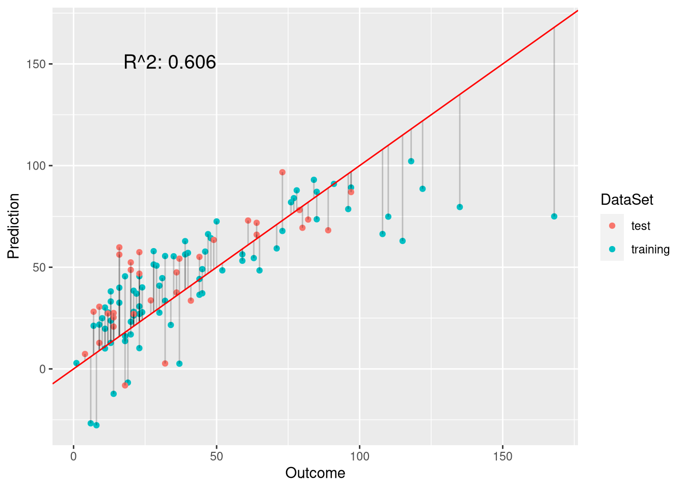
Looking at the fit of the model, there are two main observations:
- High ozone levels are underestimated
- Negative ozone levels are predicted
Let us investigate these two issues in more detail in the following.
High ozone levels are underestimated
Looking at the plot, it is noticeable that the linear model fits the outcome well when ozone is in the range [0,100]. However, when the actually observed ozone concentration is above 100, the model underpredicts the value considerably.
One question we should ask us whether these high ozone levels could not be the result of measurement errors. Considering typical ozone levels, the measured values seem reasonable. The maximal ozone level is 168 ppb (parts per billion), and 150 to 510 ppb are typical peak concentrations for US cities. This means that we should indeed be concerned with the outliers. Underestimating high ozone levels would be particularly detrimental because high levels can be health-threatening. Let us investigate the data to identify why the model has problems with these outliers.
# density of the residuals: should be normal for least-squares
plot(density(residuals(model)))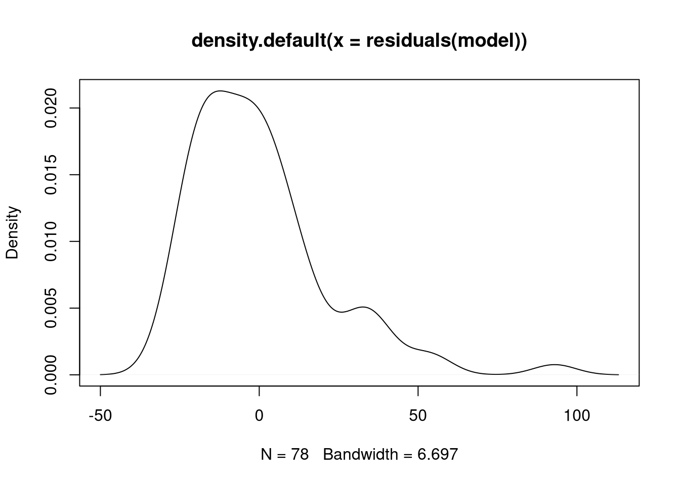
The histogram indicates that values at the right tail of the residual distribution are indeed problematic. Since the residuals are not really normally distributed, a linear model is not the best model. Indeed the residuals rather seem to follow some form of Poisson distribution. To find out why the fit of the least-squares model is so bad for the outliers, we take another look at the data.
# cutoff at 95% quantile
ozone.cut <- quantile(ozone$Ozone, 0.95)
idx <- which(ozone$Ozone >= ozone.cut)
# compare observations with high ozone with whole data set
summary(ozone[idx,])
## Ozone Solar.R Wind Temp
## Min. :110.0 Min. :207.0 Min. :2.300 Min. :79.00
## 1st Qu.:115.8 1st Qu.:223.5 1st Qu.:3.550 1st Qu.:81.75
## Median :120.0 Median :231.5 Median :4.050 Median :86.50
## Mean :128.0 Mean :236.2 Mean :4.583 Mean :86.17
## 3rd Qu.:131.8 3rd Qu.:250.8 3rd Qu.:5.300 3rd Qu.:89.75
## Max. :168.0 Max. :269.0 Max. :8.000 Max. :94.00summary(ozone)## Ozone Solar.R Wind Temp
## Min. : 1.0 Min. : 7.0 Min. : 2.30 Min. :57.00
## 1st Qu.: 18.0 1st Qu.:113.5 1st Qu.: 7.40 1st Qu.:71.00
## Median : 31.0 Median :207.0 Median : 9.70 Median :79.00
## Mean : 42.1 Mean :184.8 Mean : 9.94 Mean :77.79
## 3rd Qu.: 62.0 3rd Qu.:255.5 3rd Qu.:11.50 3rd Qu.:84.50
## Max. :168.0 Max. :334.0 Max. :20.70 Max. :97.00Looking at the distributions of the two groups of observations, we cannot see a large difference between high-ozone observations and the other samples. We can, however, find the culprit using the plot of the model predictions above. In the plot, we see that most of the data points are centered around the [0, 50] ozone range. To fit these observations well, the intercept has a large negative value of -74.19, which is why the model underestimates ozone levels for larger values of ozone, which are underrepresented in the training data.
The model predicts negative ozone levels
If the observed ozone concentration is close to 0, the model often predicts negative ozone levels. Of course, this cannot be because concentrations cannot go below 0. Again, we investigate the data to find out why the model still makes these predictions.
For this purpose, we will select all observations whose ozone level is in the 5th percentile and investigate their feature values:
# cutoff at 5% quantile
ozone.cut <- quantile(ozone$Ozone, 0.05)
idx <- which(ozone$Ozone <= ozone.cut)
# compare observations with low ozone with whole data set
summary(ozone[idx,])
## Ozone Solar.R Wind Temp
## Min. :1.0 Min. : 8.00 Min. : 9.70 Min. :57.0
## 1st Qu.:4.5 1st Qu.:20.50 1st Qu.: 9.85 1st Qu.:59.5
## Median :6.5 Median :36.50 Median :12.30 Median :61.0
## Mean :5.5 Mean :37.83 Mean :13.75 Mean :64.5
## 3rd Qu.:7.0 3rd Qu.:48.75 3rd Qu.:17.38 3rd Qu.:67.0
## Max. :8.0 Max. :78.00 Max. :20.10 Max. :80.0summary(ozone)## Ozone Solar.R Wind Temp
## Min. : 1.0 Min. : 7.0 Min. : 2.30 Min. :57.00
## 1st Qu.: 18.0 1st Qu.:113.5 1st Qu.: 7.40 1st Qu.:71.00
## Median : 31.0 Median :207.0 Median : 9.70 Median :79.00
## Mean : 42.1 Mean :184.8 Mean : 9.94 Mean :77.79
## 3rd Qu.: 62.0 3rd Qu.:255.5 3rd Qu.:11.50 3rd Qu.:84.50
## Max. :168.0 Max. :334.0 Max. :20.70 Max. :97.00What we find is that, for low ozone levels, the average solar radiation is much lower, while the average wind speed is much higher. To understand why we have negative predictions, let us now look at the model coefficients:
coefficients(model)## (Intercept) Solar.R Temp Wind
## -74.18928801 0.04506998 1.84999289 -3.34510459So, for low ozone levels, the positive coefficient for Solar.R cannot make up the negative pull of both the intercept and the coefficient for Wind because for low ozone levels, values for Solar.R are low, while values for Wind are high.
Dealing with negative ozone level predictions
Let us first deal with the problem of predicting negative ozone levels.
Truncated ordinary-least squares model
A simple approach for dealing with negative predictions is to replace them with the minimal possible value instead. In this way, if we would hand our model to a customer, he would not start suspecting that something is wrong with the model. We could do this with the following function:
predict.nonnegative <- function(model, newdata) {
   preds <- predict(model, newdata = newdata)
   # correct for negative predictions
   preds[preds < 0] <- 0
   return(preds)
}
Let us now verify how this would improve our predictions on the test data. Remember, the \(R^2\) of the initial model was was \(0.604\).
nonnegative.preds <- predict.nonnegative(model, ozone[testset,])
# plot only the test predictions to verify the results
plot.linear.model(model, nonnegative.preds, ozone$Ozone[testset], test.only = TRUE)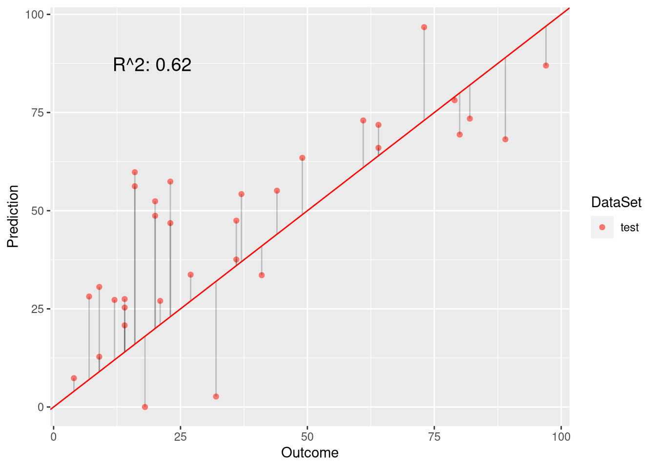
As we see, this hack curbs the problem and increases \(R^2\) to \(0.646\). However, correcting the negative values in this way, does not change the fact that our model is wrong because the fitting procedure did not take into consideration that negative values should be impossible.
Poisson regression
To prevent negative estimates, we can use of a generalized linear model (GLM) that assumes a Poisson distribution rather than a normal distribution:
pois.model <- glm(Ozone ~ Solar.R + Temp + Wind, family = "poisson",data = ozone[trainset, ])
# need to set type to 'response' to get exponentiated predictions
pois.preds <- predict(pois.model, newdata = ozone[testset,], type = "response")
plot.linear.model(pois.model, pois.preds, ozone$Ozone[testset])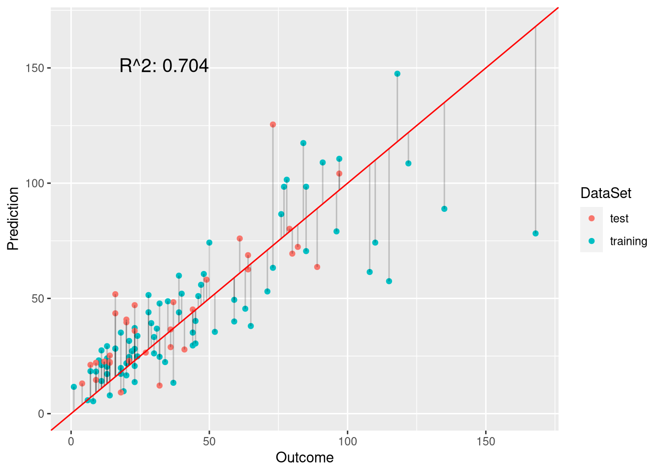
The \(R^2\) value of 0.616 indicates that Poisson regression is slightly superior over ordinary least-squares (0.604). However, its performance is not superior to the model that truncates negative values to 0 (0.646). This is probably because the variance of the ozone level is much larger than what the Poisson model assumes:
# mean and variance should be the same for Poisson distribution
mean(ozone$Ozone)
## [1] 42.0991var(ozone$Ozone)## [1] 1107.29Logarithm transformation
Another approach for dealing with negative predictions is taking the logarithm of the outcome:
log.model <- lm(log(Ozone) ~ Solar.R + Temp + Wind, ozone, trainset)
log.preds <- predict(pois.model, newdata = ozone[testset,], type = "response")
print(rsquared(log.preds, test.labels))
## [1] 0.704Note that although the result is identical to the result via Poisson regression, the two methods are not identical in general.
Dealing with the underestimation of high ozone levels
Ideally, we would have a better sampling of measurements with high ozone levels. However, since we cannot collect more data, we need to make do with what we have. One way to deal with the underestimation of high ozone levels is adjusting the loss function.
Weighted regression
Using weighted regression, we can influence the impact of the residuals of the outliers. For this purpose, we will calculate the z-scores of the ozone levels and then use their exponential as the weight for the model such that the impact of outliers is increased.
get.weights <- function(ozone) {
    z.scores <- (ozone$Ozone - mean(ozone$Ozone)) / sd(ozone$Ozone)
    weights <- exp(z.scores)
    weights <- weights / mean(weights) # normalize to mean 1
    return(weights)
}
weights <- get.weights(ozone)
weight.model <- lm(Ozone ~ Solar.R + Temp + Wind, ozone, trainset, weights = weights)
weight.preds <- predict(weight.model, newdata = ozone[testset,], type = "response")
plot.linear.model(weight.model, weight.preds, ozone$Ozone[testset])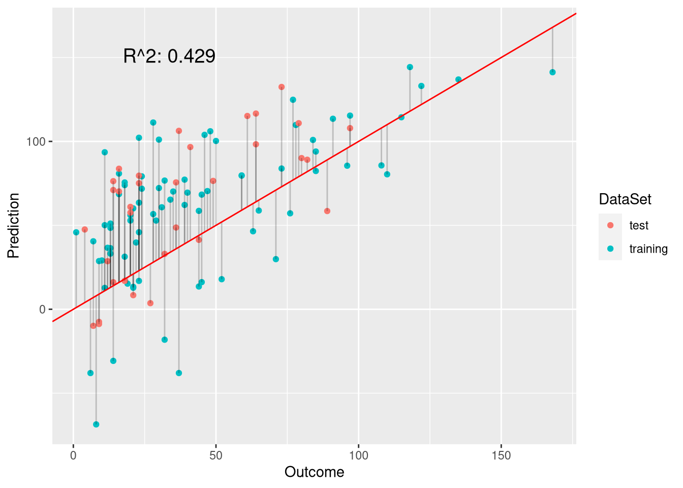
This model is definitely more appropriate than the ordinary least-squares model as it deals better with the outliers.
Sampling
Let’ sample from the training data such that high ozone levels are not underrepresented anymore. This is simlar to doing weighted regression. However, rather than setting small weights to the observations with low ozone levels, we implicitly set their weights to 0.
# randomly discard 50% of samples with ozone < 50 because these are overrepresented
discard.ratio <- 0.5
low.ozone.idx <- which(ozone$Ozone[trainset] < 50)
n.discard <- ceiling(discard.ratio * length(low.ozone.idx))
discard.idx <- sample(trainset[low.ozone.idx], n.discard)
print(paste0("N (trainset before): ", length(trainset)))
## [1] "N (trainset before): 78"trainset.sampled <- setdiff(trainset, discard.idx)
print(paste0("N (trainset after): ", length(trainset.sampled)))## [1] "N (trainset after): 51"Now, let us build a new model based on the sampled data:
# performance is not much bettter for test set
sampled.model <- glm(Ozone ~ Solar.R + Temp + Wind, data = ozone[trainset.sampled, ])
sampled.preds <- predict(sampled.model, newdata = ozone[testset,], type = "response")
rsquared(sampled.preds, test.labels)
## [1] 0.608As we can see, the model based on the sampled data does not perform better than the one using weights.
Combining the evidence
Having seen that Poisson regression is useful for preventing negative estimates and that weighting is a successful strategy for improving the prediction of outliers, we should try to combine both approaches, which leads to weighted Poisson regression.
Weighted Poisson regression
w.pois.model <- glm(Ozone ~ Solar.R + Temp + Wind, ozone, trainset,
                    weights = weights, family = "poisson")
w.pois.preds <- predict(w.pois.model, newdata = ozone[testset,], type = "response")
p.w.pois <- plot.linear.model(w.pois.model, w.pois.preds, ozone$Ozone[testset])
p.w.pois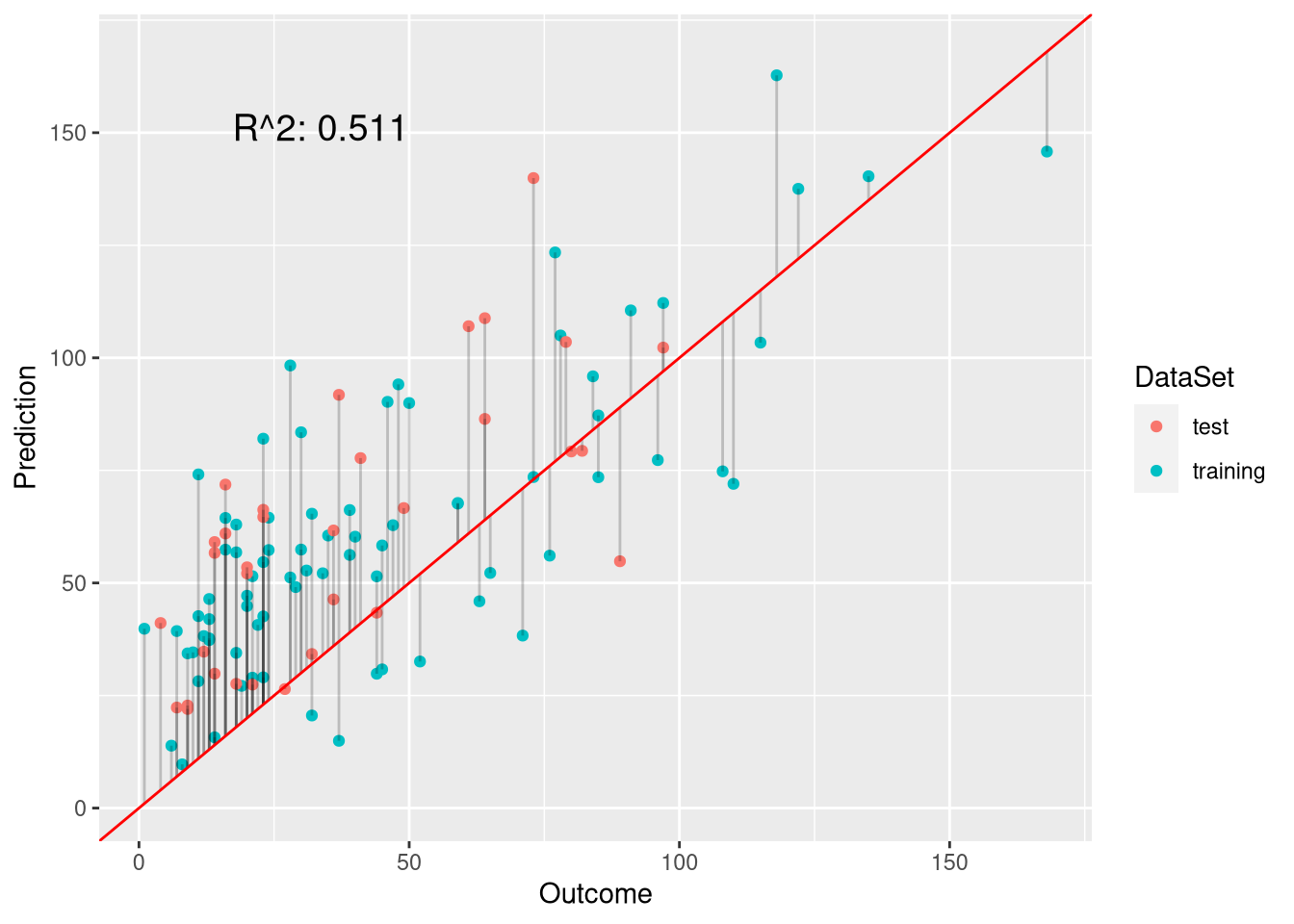
As we see, this model combines the advantages of using Poisson regression (non-negative predictions) with the use of weights (underestimation of outliers). Indeed, the \(R^2\) of this model is the lowest yet (0.652 vs 0.646 from the truncated linear model). Let us investigate the model coefficients:
coefficients(w.pois.model)## (Intercept) Solar.R Temp Wind
## 5.074448971 0.001987798 -0.001202156 -0.137611701The model is still dominated by the intercept but now it is positive. Thus, if all other features have a value of 0, the prediction of the model will still be positive.
However, what about the assumption that the mean should be equal to the variance for Poisson regression?
print(paste0(c("Var: ", "Mean: "), c(round(var(ozone$Ozone), 2),
        round(mean(ozone$Ozone), 2))))
## [1] "Var: 1107.29" "Mean: 42.1"The assumption of the model is definitely not met and we suffer from overdispersion since the variance is greater than assumed by the model.
Weighted negative binomial model
So, we should try picking a model that is more suitable for overdispersion such as the negative binomial model:
library(MASS)
# train weighted negative binomial model
model.nb <- glm.nb(Ozone ~ Solar.R + Temp + Wind, data = ozone, subset = trainset, weights = weights)
preds.nb <- predict(model.nb, newdata = ozone[testset,], type = "response")
plot.linear.model(model.nb, preds.nb, test.labels)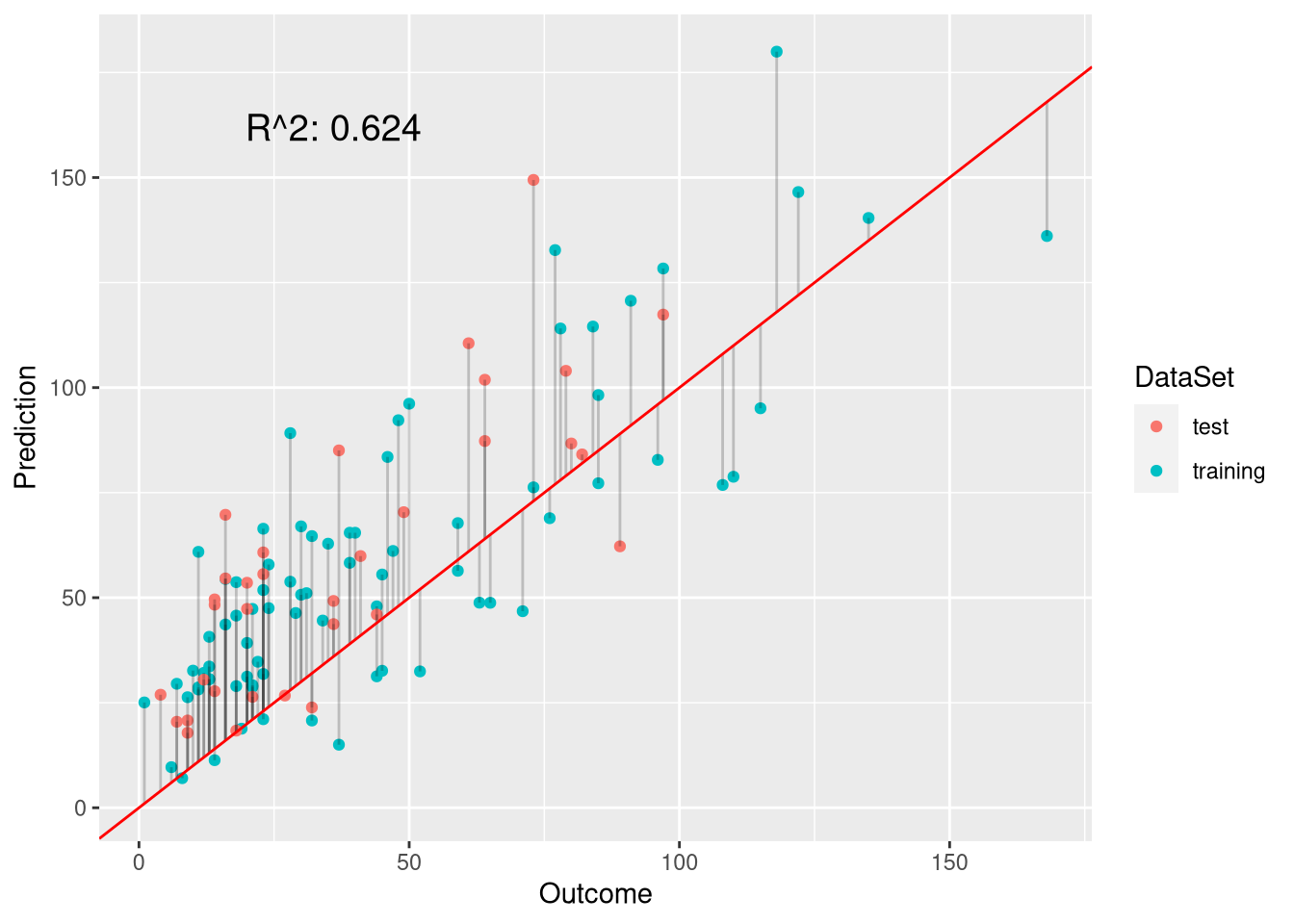
So, in terms of performance on the test set, the weighted negative binomial model is not better thatn the weighted Poisson model. However, when it comes to inference, the value should be superior because its assumptions are not broken. Looking at both models, it is evident that their p-values differ considerably:
coef(summary(w.pois.model))## Estimate Std. Error z value Pr(>|z|)
## (Intercept) 5.074448971 0.1668873283 30.4064366 4.515679e-203
## Solar.R 0.001987798 0.0002630893 7.5556013 4.169292e-14
## Temp -0.001202156 0.0017067486 -0.7043545 4.812120e-01
## Wind -0.137611701 0.0042937826 -32.0490610 2.262476e-225coef(summary(model.nb))## Estimate Std. Error z value Pr(>|z|)
## (Intercept) 3.651242295 0.4874400886 7.490648 6.853421e-14
## Solar.R 0.002591735 0.0006855076 3.780752 1.563551e-04
## Temp 0.013312402 0.0052097134 2.555304 1.060950e-02
## Wind -0.127395396 0.0113987431 -11.176267 5.328447e-29While the Poisson model claims that all coefficients are highly significant, the negative binomial model demonstrates that the intercept is not significant. As described nicely in this blog and at StackExchange, the confidence bands for a negative binomial can be found in the following way:
# predict on the link level, which is more Gaussian:
preds.nb.ci <- predict(model.nb, newdata = ozone[testset, ], type = "link", se.fit = TRUE)
# compute confidence intervals
ilink <- family(model.nb)$linkinv # exponential
## parameters of the negative binomial
theta <- model.nb$theta # 'r' parameter of negative binomial (nbr of successes)
mu <- preds.nb.ci$fit # mean of negative binomial varies per fitted point
p <- theta / (theta + mu) # probability of success parametrization of negative binomial
# find 95% CI for normal distribution
# (we're not taking these values from the negative binomial because SEs are for normal distribution)
# ci.factor <- qnbinom(1 - (1 - CI.int)/2, size = theta, mu = as.numeric(preds.nb.ci$fit)) # different factors per observation
ci.factor <- 1.96
CI.int <- 0.95
# calculate CIs:
df <- data.frame(ozone[testset,], "PredictedOzone" = ilink(preds.nb.ci$fit), "Lower" = ilink(preds.nb.ci$fit - ci.factor * preds.nb.ci$se.fit),
                "Upper" = ilink(preds.nb.ci$fit + ci.factor * preds.nb.ci$se.fit))
Using the constructed data frame containing the values of the features in the test set as well as the predictions with their confidence bands, we can plot how the estimates fluctuate in dependence on the independent variables:
# plot estimates vs individual features in the test set
plots <- list()
for (feature in colnames(ozone)) {
    if (feature == "Ozone") {
        next
    }
    p <- ggplot(df, aes_string(x = feature,
                       y = "PredictedOzone")) +
      geom_line(colour = "blue") +
      geom_point() +
      geom_ribbon(aes(ymin = Lower, ymax = Upper),
                    alpha = 0.5)
      plots[[feature]] <- p
}
library(gridExtra)
grid.arrange(plots[[1]], plots[[2]], plots[[3]])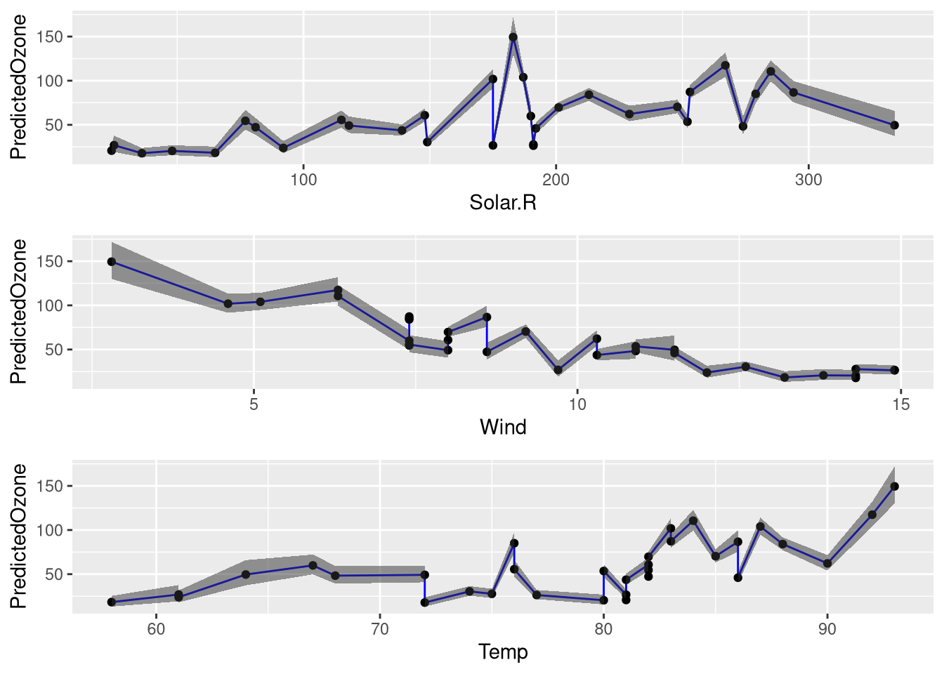
These plots demonstrate two things:
- There are clear linear relationships for
WindandTemperature. Estimated ozone levels drop whenWindincreases, while estimated ozone levels increase whenTempincreases. - The model is most confident for low ozone levels but less confident for high ozone levels
Data set augmentation
Having optimized the model, we now go back to the initial data set. Remember that we have removed all observations with missing values at the beginning of the analysis? Well, this is not ideal because we have discarded valuable information, which could be used to obtain a better model.
Investigating the missing values
Let us first investigate the missing values:
data(airquality)
# store old ozone data set
ozone.old <- ozone
# remove time-specific features
ozone <- subset(airquality, select = c("Ozone", "Solar.R", "Wind", "Temp"))
# select observations with missing values
na.idx <- as.numeric(which(apply(is.na(ozone),1, any)))
na.df <- ozone[na.idx, ]
# ratio of missing values
ratio.missing <- length(na.idx) / nrow(ozone)
print(paste0(round(ratio.missing * 100, 3), "%"))
## [1] "27.451%"# which features are missing most often?
nbr.missing <- apply(ozone, 2, function(x) length(which(is.na(x))))
print(nbr.missing)## Ozone Solar.R Wind Temp
## 37 7 0 0# multiple features missing in one observation?
nbr.missing <- apply(ozone, 1, function(x) length(which(is.na(x))))
table(nbr.missing)## nbr.missing
## 0 1 2
## 111 40 2The investigation reveals that a considerable percentage of observations were previously excluded due to missing values. More specifically, the only features that are missing are Ozone (37 times) and Solar.R (7 times). Usually, only one feature is missing (40 times) and rarely are two features missing (2 times).
Adjusting training and test indices
To ensure that the same observations are used for testing as previously, we have to remap the old incies to the full airquality data set:
## ensure that same observations are used for testing again:
# adjust training/test indices for the new data set
old.trainset <- trainset
trainset <- match(rownames(ozone.old)[old.trainset], rownames(ozone))
# add NA observations to training data set
trainset <- c(trainset, na.idx)
testset <- setdiff(seq_len(nrow(ozone)), trainset)
Imputing missing values
To obtain estimates of the missing values, we can use imputation. The idea of this approach is to form predictive models using the known features in order to estimates the missing features. In this way, no observations have to be discarded. When imputing values, it is important that the test data are not used because this would defeat its purpose (the test set would not be independent of the model anymore).
# use Hmisc for imputing missing values
library(Hmisc)
# use aregImpute for multiple imputation
imputed <- aregImpute(Ozone ~ Solar.R + Temp + Wind, ozone, pr = FALSE)
# list.out: return a list; imputation: arbitrarily use the first imputation
imputed.data <- as.data.frame(impute.transcan(imputed, data = ozone,
                imputation = 1, list.out = TRUE,  pr = FALSE))
# inspect imputed observations with respect to the outcome
summary(as.numeric(imputed.data$Ozone))
## Min. 1st Qu. Median Mean 3rd Qu. Max.
## 1.00 18.00 31.00 41.38 63.00 168.00Note that aregImpute makes several multiple imputations with different bootstrap samples, which can be specified using the n.impute parameter. Since we want to use the imputations from all runs rather than a single one, we will use the fit.mult.impute function to define our model:
# compute new weights
weights <- get.weights(imputed.data)
# use imputations from all iterations rather than an arbitrary iteration:
fmi <- fit.mult.impute(Ozone ~ Solar.R + Temp + Wind,
        fitter=glm, xtrans = imputed, family = "poisson",
        data = ozone, subset = trainset, pr = FALSE) #, weights = weights)
        # weights arguments (weights = weights) not used due to error:
        # "..2 used in an incorrect context, no ... to look in"
fmi.preds <- predict.glm(fmi, newdata = ozone[testset,], type = "response")
plot.linear.model(fmi, fmi.preds, ozone$Ozone[testset])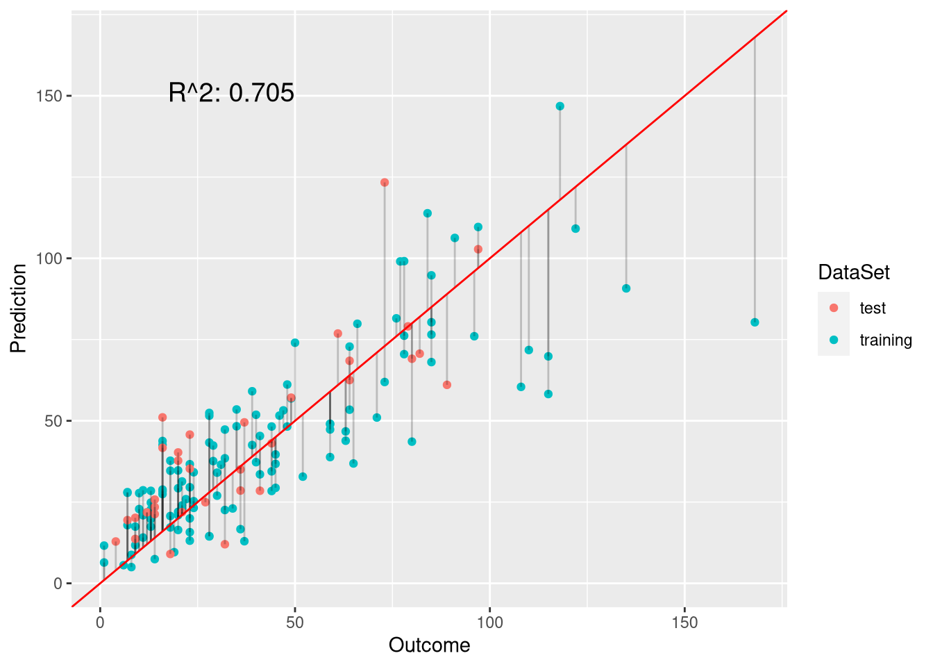
Let us use just a single imputation in order to specify the weights again:
w.pois.model.imputed <- glm(Ozone ~ Solar.R + Temp + Wind, imputed.data,
                        trainset, weights = weights, family = "poisson")
w.pois.preds.imputed <- predict(w.pois.model.imputed,
                newdata = imputed.data[testset,], type = "response")
rsquared(w.pois.preds.imputed, imputed.data$Ozone[testset])
## [1] 0.592In this case, the weighted Poisson model based on imputed data did not perform better than the model that simply excluded missing data. This indicates that imputation of the missing values rather introduces noise into the data than signal we can work with. A possible explanation would be that the samples with missing values have another distribution than the values for which all measurements are available.
Summary
We started with an OLS regression model (\(R^2 = 0.604\)) and tried to find a linear model with a better fit. The first idea was to truncate the predictions of the model at 0 (\(R^2 = 0.646\)). To predict outliers more accurately, we trained a weighted linear regression model (\(R^2 = 0.621\)). Next, to predict only positive values, we trained a weighted Poisson regression model (\(R^2 = 0.652\)). To deal with the problem of overdispersion in the Poisson model, we formulated a weighted negative binomial model. Although this model perfomed worse than the weighted Poisson model (\(R^2 = 0.638\)), it is likely to be superior for making inferences.
Thereafter, we tried to further improve the model by imputing missing values with the Hmisc package. Although the resulting models were better than the initial OLS model, they did not obtain a higher performance than previously (\(R^2 = 0.627\)).
So, what is the best model in the end? In terms of correctness of the model assumptions this is the weighted negative binomial model. In terms of the coefficient of determination, \(R^2\), this is the weighted Poisson regression model. So, for the purpose of predicting ozone levels, I would select the weighted Poisson regression model.
You may ask: was all this work worth the effort? Indeed, the the predictions of the initial model and the weighted Poisson model are significantly different at the 5% level:
# does the new model predict significantly different values?
wilcox.test(test.preds, w.pois.preds, paired = TRUE)
##
## Wilcoxon signed rank exact test
##
## data: test.preds and w.pois.preds
## V = 70, p-value = 6.212e-05
## alternative hypothesis: true location shift is not equal to 0The difference between the models becomes obvious when we compare them side-by-side:
library(gridExtra) # for grid.arrange
library(grid) # for textGrob function
grid.arrange(p.OLS, p.w.pois, nrow = 1, top=textGrob("Ordinary least squares vs weighted Poisson regression",gp=gpar(fontsize=20,font=3)))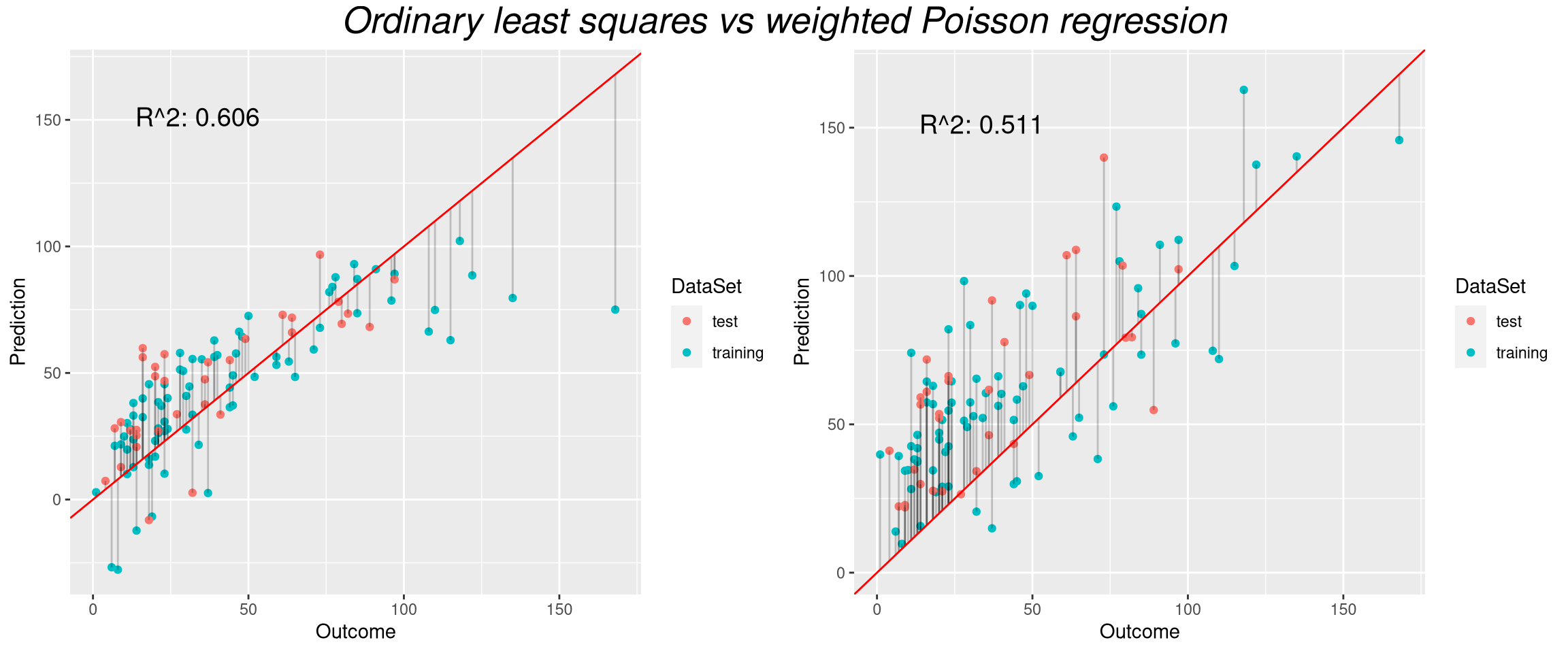
In conclusion, we went from a model that predicted negative values and underestimated high ozone levels (the OLS model shown on the left) to a model that has no such apparent shortcomings (the weighted Poisson model on the right).
Note that the whole analysis is limited by the fact that we evaluated performance on a single test set. Using cross-validation, which averages out the randomness of selecting a specific test set, the observed model performance would be different. One should especially not obsess about the performance on a test set that is as small as the current one (n = 33), since a high performance on such a small test set does not necessarily give rise to high generalizability.


Comments
There aren't any comments yet. Be the first to comment!