Comparing Medians and Inter-Quartile Ranges Using the Box Plot
Creating a box plot in native R
We will use the warpbreaks data set to exemplify the use of box plots. In native R, a box plot can be obtained via boxplot.
data(warpbreaks)
# create positions for tick marks, one more than number of bars
x <- warpbreaks$breaks
# create labels
x.labels <- paste0(warpbreaks$wool, "-", warpbreaks$tension)
# specify colors for groups
group.cols <- c("darkred", "red", "darksalmon",
                "darkblue", "blue", "lightblue")
cols <- c(rep(group.cols[1], 9), rep(group.cols[2], 9),
        rep(group.cols[3], 9), rep(group.cols[4], 9),
        rep(group.cols[5], 9), rep(group.cols[6], 9))
boxplot(x ~ warpbreaks$wool + warpbreaks$tension, col = group.cols)
legend("topright", legend = c(unique(x.labels)),
        col = group.cols, pch = 20)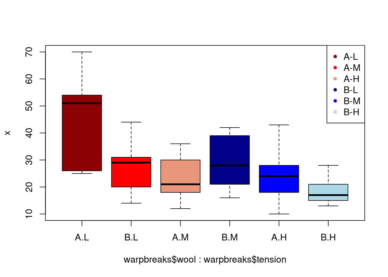
Creating a box plot with ggplot
We could compare the tensions for each type of wool using facet_wrap in the following way:
library(ggplot2)
ggplot(warpbreaks, aes(x = tension, y = breaks)) +
    geom_boxplot() + facet_wrap(.~wool) +
    ggtitle("Breaks for wool A and B")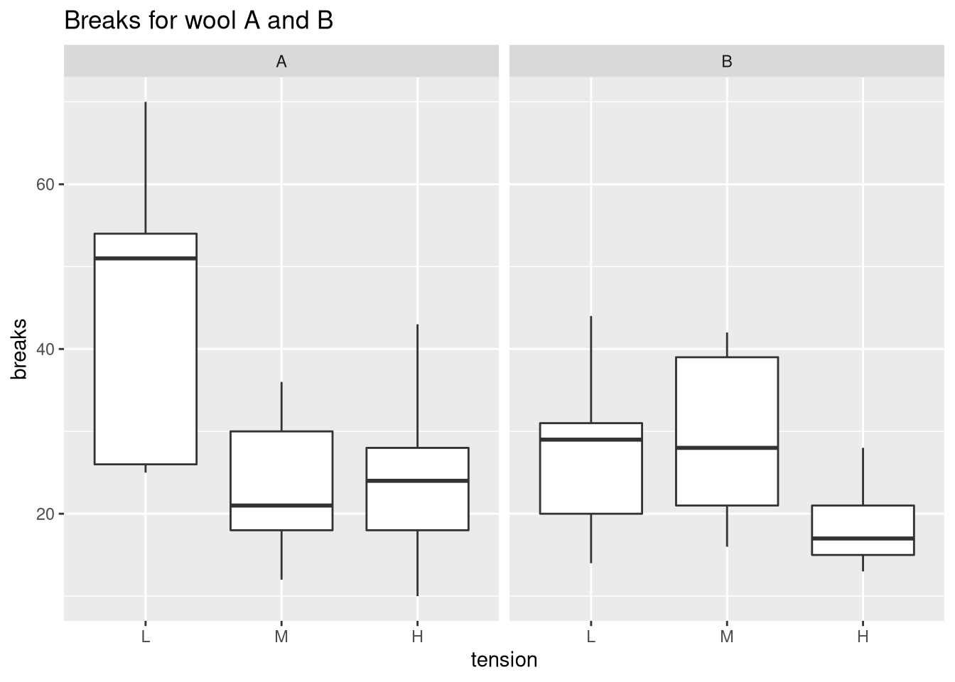
ggplot(warpbreaks, aes(x = tension, y = breaks, fill = wool)) +
    geom_boxplot() +
    ggtitle("Breaks for wool A and B")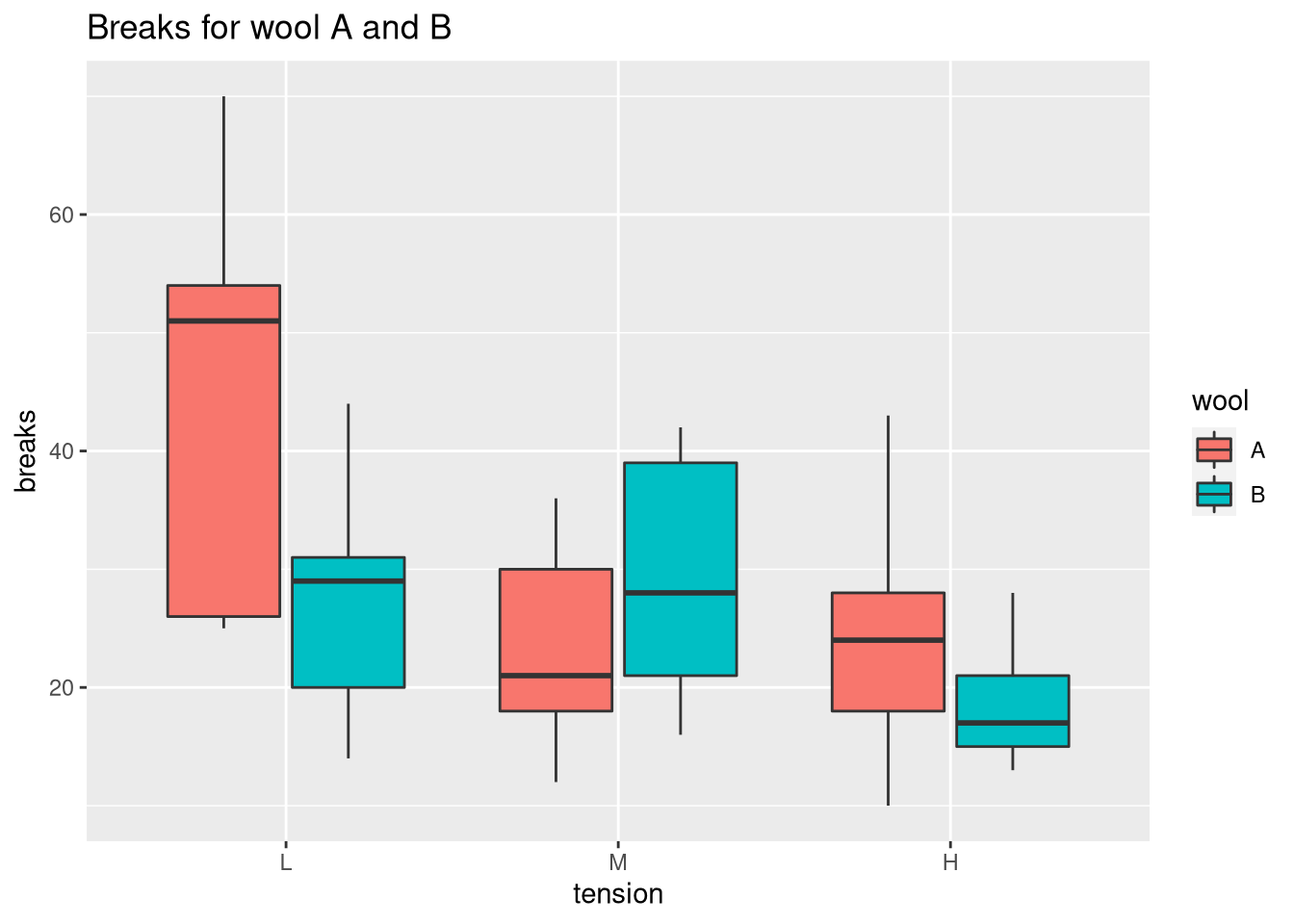
Showing all points
To view the individual measurements associated with the box plot, we set outlier.shape = NA to prevent duplicates and call geom_point.
ggplot(warpbreaks, aes(x = tension, y = breaks, fill = wool)) +
    geom_boxplot(outlier.shape = NA) +
    ggtitle("Breaks for wool A and B") +
    # dodge points horizontally (there are two bars per tick)
    # and jitter points horizontally so that they don't overlap
    geom_point(position = position_jitterdodge(jitter.width = 0.1))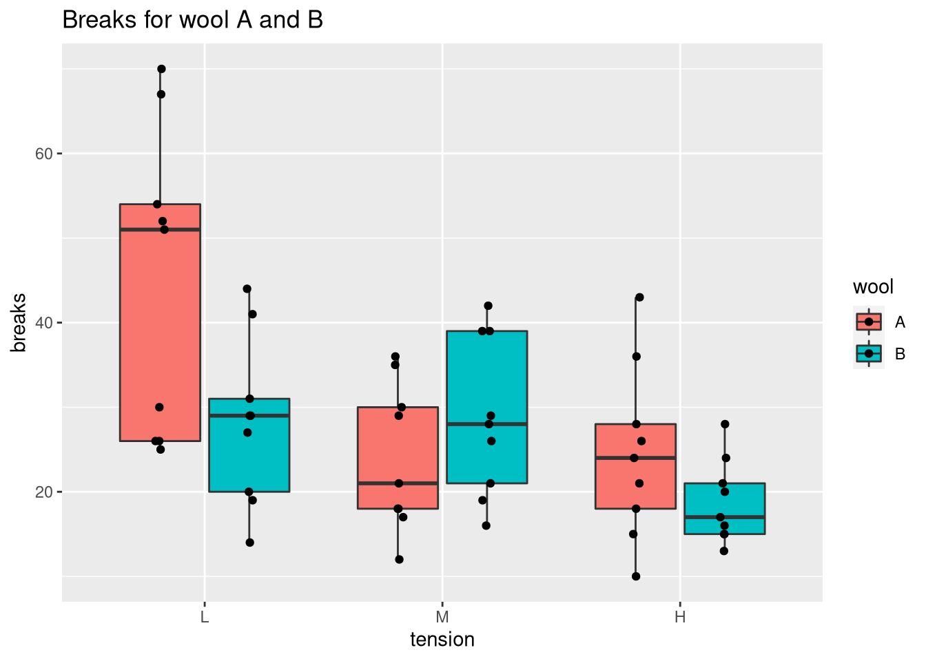
Showing all the points helps us to identify whether the sample size is sufficient. In this case, most pairs of wool and tension exhibit high variabilities (especially wool A with tension L). Thus, the question would be whether this level of variability is inherent to the data or a result of the small number of samples (n = 9). Note that you can combine a box plot with a beeswarm plot to optimize the locations of the points.


Comments
There aren't any comments yet. Be the first to comment!