Using probability distributions in R: dnorm, pnorm, qnorm, and rnorm

Distribution functions in R

Every distribution has four associated functions whose prefix indicates the type of function and the suffix indicates the distribution. To exemplify the use of these functions, I will limit myself to the normal (Gaussian) distribution. The four normal distribution functions are:

• dnorm: density function of the normal distribution
• pnorm: cumulative density function of the normal distribution
• qnorm: quantile function of the normal distribution
• rnorm: random sampling from the normal distribution

The probability density function: dnorm

The probability density function (PDF, in short: density) indicates the probability of observing a measurement with a specific value and thus the integral over the density is always 1. For a value \(x\), the normal density is defined as \[{\displaystyle f(x\mid \mu ,\sigma ^{2})={\frac {1}{\sqrt {2\pi \sigma ^{2}}}}\text{exp}\left(-{\frac {(x-\mu )^{2}}{2\sigma ^{2}}}\right)}\] where \(\mu\) is the mean, \(\sigma\) is the standard deviation, and \(\sigma^2\) is the variance.

Using the density, it is possible to determine the probabilities of events. For example, you may wonder: What is the likelihood that a person has an IQ of exactly 140?. In this case, you would need to retrieve the density of the IQ distribution at value 140. The IQ distribution can be modeled with a mean of 100 and a standard deviation of 15. The corresponding density is:

sample.range <- 50:150
iq.mean <- 100
iq.sd <- 15
iq.dist <- dnorm(sample.range, mean = iq.mean, sd = iq.sd)
iq.df <- data.frame("IQ" = sample.range, "Density" = iq.dist)
library(ggplot2)
ggplot(iq.df, aes(x = IQ, y = Density)) + geom_point()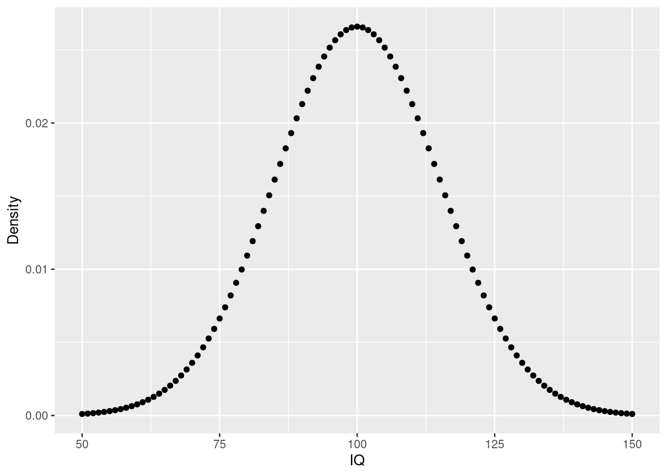

From these data, we can now answer the initial question as well as additional questions:

pp <- function(x) {
    print(paste0(round(x * 100, 3), "%"))
}
# likelihood of IQ == 140?
pp(iq.df$Density[iq.df$IQ == 140])

## [1] "0.076%"

# likelihood of IQ >= 140?
pp(sum(iq.df$Density[iq.df$IQ >= 140]))

## [1] "0.384%"

# likelihood of 50 < IQ <= 90?
pp(sum(iq.df$Density[iq.df$IQ <= 90]))

## [1] "26.284%"

The cumulative density function: pnorm

The cumulative density (CDF) function is a monotonically increasing function as it integrates over densities via \[f(x | \mu, \sigma) = \displaystyle {\frac {1}{2}}\left[1+\operatorname {erf} \left({\frac {x-\mu }{\sigma {\sqrt {2}}}}\right)\right]\] where \(\text{erf}(x) = \frac {1}{\sqrt {\pi }}\int _{-x}^{x}e^{-t^{2}}\,dt\) is the error function.

To get an intuition of the CDF, let’s create a plot for the IQ data:

cdf <- pnorm(sample.range, iq.mean, iq.sd)
iq.df <- cbind(iq.df, "CDF_LowerTail" = cdf)
ggplot(iq.df, aes(x = IQ, y = CDF_LowerTail)) + geom_point()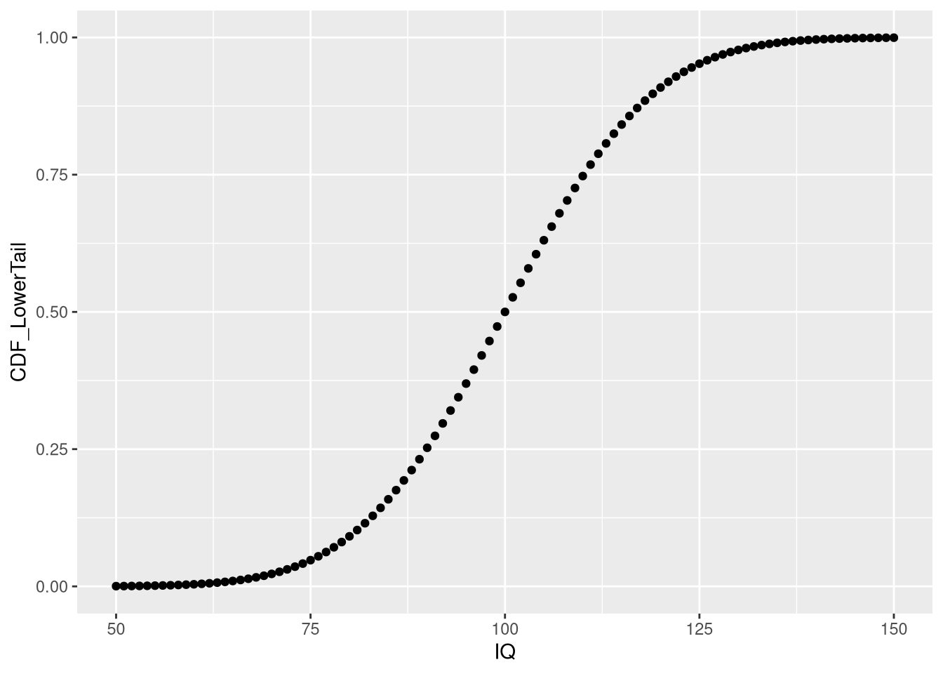

As we can see, the depicted CDF shows the probability of having an IQ less or equal to a given value. This is because pnorm computes the lower tail by default, i.e. \(P[X <= x]\). Using this knowledge, we can obtain answers to some of our previous questions in a slightly different manner:

# likelihood of 50 < IQ <= 90?
pp(iq.df$CDF_LowerTail[iq.df$IQ == 90])

## [1] "25.249%"

# set lower.tail to FALSE to obtain P[X >= x]
cdf <- pnorm(sample.range, iq.mean, iq.sd, lower.tail = FALSE)
iq.df <- cbind(iq.df, "CDF_UpperTail" = cdf)
# Probability for IQ >= 140? same value as before using dnorm!
pp(iq.df$CDF_UpperTail[iq.df$IQ == 140])

## [1] "0.383%"

Note that the results from pnorm are the same as those obtained from manually summing up the probabilities obtained via dnorm. Moreover, by setting lower.tail = FALSE, dnorm can be used to directly compute p-values, which measure how the likelihood of an observation that is at least as extreme as the obtained one.

To remember that pnorm does not provide the PDF but the CDF, just imagine that the function carries a p in its name such that pnorm is lexicographically close to qnorm, which provides the inverse of the CDF.

The quantile function: qnorm

The quantile function is simply the inverse of the cumulative density function (iCDF). Thus, the quantile function maps from probabilities to values. Let’s take a look at the quantile function for \(P[X <= x]\):

# input to qnorm is a vector of probabilities
prob.range <- seq(0, 1, 0.001)
icdf.df <- data.frame("Probability" = prob.range, "IQ" = qnorm(prob.range, iq.mean, iq.sd))
ggplot(icdf.df, aes(x = Probability, y = IQ)) + geom_point()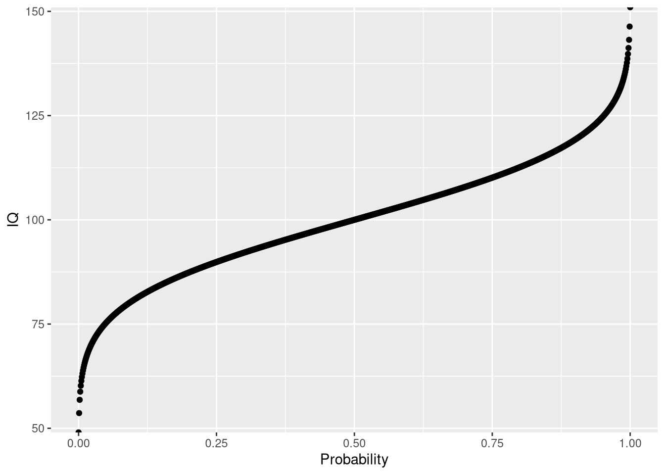

Using the quantile function, we can answer quantile-related questions:

# what is the 25th IQ percentile?
print(icdf.df$IQ[icdf.df$Probability == 0.25])

## [1] 89.88265

# what is the 75 IQ percentile?
print(icdf.df$IQ[icdf.df$Probability == 0.75])

## [1] 110.1173

# note: this is the same results as from the quantile function
quantile(icdf.df$IQ)

##        0%       25%       50%       75%      100% 
##      -Inf  89.88265 100.00000 110.11735       Inf

The random sampling function: rnorm

When you want to draw random samples from the normal distribution, you can use rnorm. For example, we could use rnorm to simulate random samples from the IQ distribution.

# fix random seed for reproducibility
set.seed(1)
# law of large numbers: mean will approach expected value for large N
n.samples <- c(100, 1000, 10000)
my.df <- do.call(rbind, lapply(n.samples, function(x) data.frame("SampleSize" = x, "IQ" = rnorm(x, iq.mean, iq.sd))))
# show one facet per random sample of a given size
ggplot() + geom_histogram(data = my.df, aes(x = IQ)) + facet_wrap(.~SampleSize, scales = "free_y")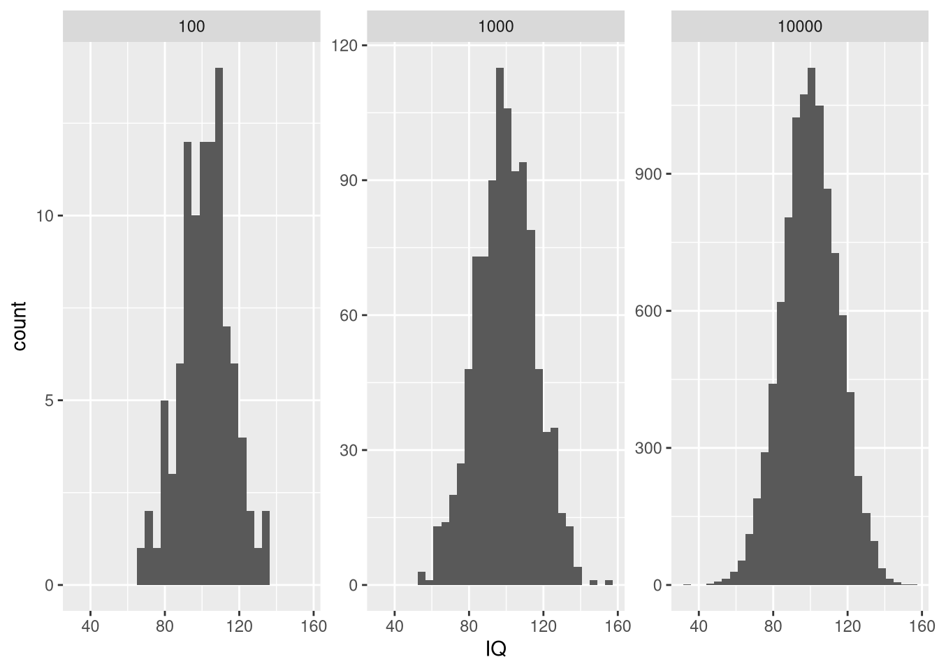

# note: we can also implement our own sampler using the densities
my.sample <- sample(iq.df$IQ, 100, prob = iq.df$Density, replace = TRUE)
my.sample.df <- data.frame("IQ" = my.sample)
ggplot(my.sample.df, aes(x = IQ)) + geom_histogram()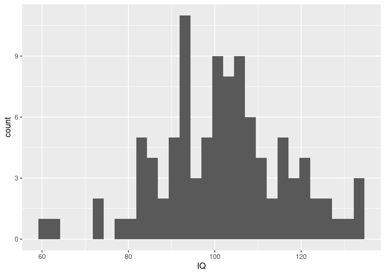

Note that we called set.seed in order to ensure that the random number generator always generates the same sequence of numbers for reproducibility.

Summary

Of the four functions dealing with distributions, dnorm is the most important one. This is because the values from pnorm, qnorm, and rnorm are based on dnorm. Still, pnorm, qnorm, and rnorm are very useful convenience functions when dealing with the normal distribution. If you would like to learn about the corresponding functions for the other distributions, you can simply call ?distribtuion to obtain more information.