Parametric Testing: How Many Samples Do I Need?
Fitting normal distributions to sampled means
To investigate the number of samples that are necessary to satisfy the requirements for Student’s t-test, we iterate over various sample sizes. For each sample size, we draw samples from several distributions. Then, the means of the samples are calculated and a normal distribution is fitted to the distribution of the means. In each iteration, we record the log-likelihood describing how well the normal distribution fits the sampled means. We’ll consider sampled means to have approached the normal distribution when the log likelihood becomes positive.
require(MASS)
require(reshape2)
require(ggplot2)
# set seed to ensure that results are reproducible
set.seed(5)
nbr.samples <- 500
sample.sizes <- c(5, 10, 15, 20, 50, 100, 1000, 5000)
result <- NULL
initial.means <- NULL
norm.means <- list()
for (i in seq_along(sample.sizes)) {
    sample.size <- sample.sizes[i]
    beta.data <- sapply(rep(sample.size, nbr.samples), rbeta, 1,5)
    norm.data <- sapply(rep(sample.size,nbr.samples),rnorm)
    chi.data <- sapply(rep(sample.size,nbr.samples),rchisq,df=1)
    pois.data <- sapply(rep(sample.size,nbr.samples),rpois, lambda = 5)
    student.data <- sapply(rep(sample.size, nbr.samples), rt, df = 1)
    all.data <- list("Beta" = beta.data, "Normal" = norm.data, "Chi" = chi.data, "Poisson" = pois.data, "Student" = student.data)
    means <- lapply(all.data, colMeans)
    # store initial mean distribution for visualization
    if (i == 1) {
        initial.means <- means
    }
    logliks <- lapply(means, function(x) fitdistr(x, densfun = "normal")$loglik)
    positive.lik <- names(logliks)[which(logliks > 0)]
    positive.lik <- positive.lik[!positive.lik  %in% names(norm.means)]
    # store as first normal distribution for visualization
    norm.means[positive.lik] <- means[positive.lik]
    result <- rbind(result, data.frame("Sample_Size" = sample.size, logliks))
}
Log likelihoods of fits
Investigating the results, we can see that some distributions seem to approach the normal distribution faster than others:
print(result)## Sample_Size Beta Normal Chi Poisson Student
## 1 5 694.9139 -299.81161 -496.33474 -702.94076 -1971.203
## 2 10 823.0384 -126.68806 -297.08253 -515.18702 -3806.447
## 3 15 909.4417 -30.63266 -199.77525 -455.64737 -2119.944
## 4 20 1045.1414 46.45709 -136.21868 -375.75690 -2263.025
## 5 50 1235.7655 278.66189 84.44694 -117.56140 -3427.721
## 6 100 1397.7265 443.81523 281.68706 47.87537 -2178.871
## 7 1000 1996.2198 1019.70692 845.26837 619.25871 -3636.674
## 8 5000 2398.4267 1402.41433 1260.47873 1018.24454 -3231.983According to positive log likelihoods, the beta distribution yields normally distributed means already at a sample size of 5. Normal, chi-squared, and Poisson distributions yield normally distributed means at sample sizes of 20, 50, and 100, respectively. Finally, the means of Student’s distribution never become normal since the distribution with one degree of freedom has infinite kurtosis (very heavy tails) such that the central limit theorem does not hold.
Verifying the log-likelihood criterion
As verification of the results, let’s plot the histograms at the sample size of 5 and at the sample size where the mean distribution became normal:
plot.means <- function(means) {
    mean.df <- as.data.frame(means)
    mean.df <- melt(mean.df, id.vars = NULL)
    ggplot(mean.df, aes(x = value)) + geom_histogram(bins = 100) + facet_wrap(.~variable, scales = "free_x")
}
plot.means(initial.means)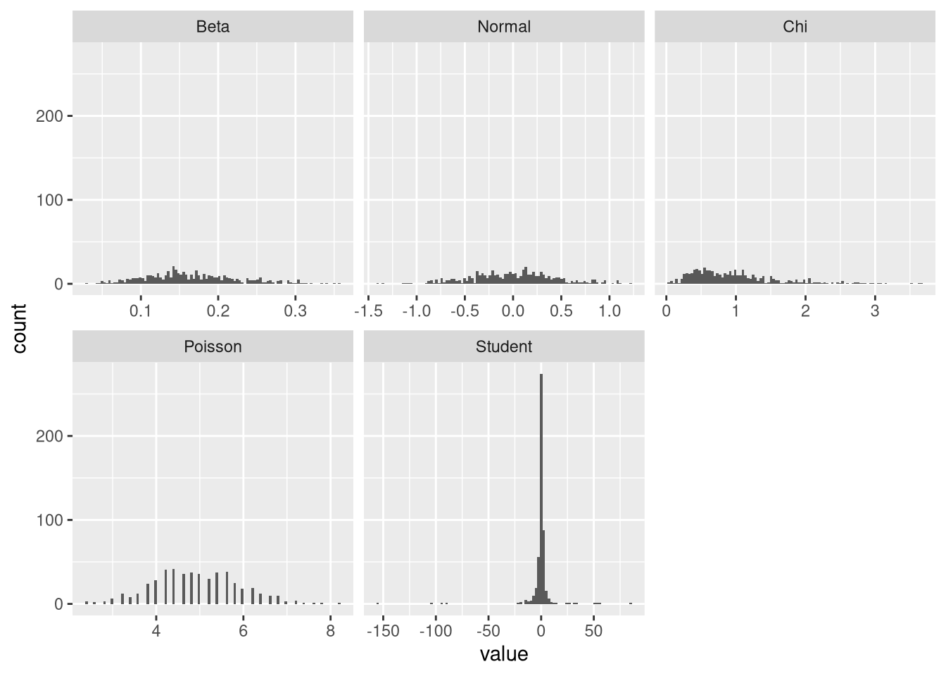
plot.means(norm.means)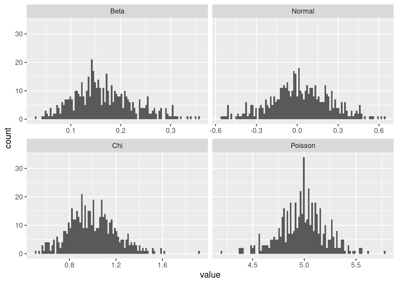
These results indicate that the log-likelihood criterion is a sufficient proxy for normality. Note, however, that from visual inspection, the initial beta distribution of means does not seem more normal than the one arising from the normal distribution. So this result may be taken with a grain of salt. Looking at Student’s t-distribution, we can see why it its means are not normally distributed:
round(quantile(means$Student), 2)## 0% 25% 50% 75% 100%
## -495.61 -0.95 0.00 0.98 3422.66For some of the samples, the mean distribution has extreme outliers at both tails of the distribution.
Conclusions
The results of these experiments indicate that Student’s t-test should definitely be avoided for sample sizes smaller than 20. The assumptions of the test seem to be met for most distribution when the sample size is at least 100. So, it turns out I was correct in having a bad feeling when I recently applied the t-test on only 10 samples.
To conclude, it is particularly advisable to check the distribution of the measurements for sample sizes below 100. Since the central limit theorem does not hold for distributions with infinite variance, it is also reasonable to verify the distribution of measurements for large sample sizes in order to exclude the possibility of such a distribution. As we have seen here, measurements distributed according to the t-distribution with one degree of freedom did not fulfill the assumption of the test even at a sample size of 5000.
So, at what sample size do you feel confident using parametric tests such as Student’s t-test? When do you investigate the distribution of the data?
This post was inspired by this discussion at Stack Exchange. A further discussion of infinite variance can be found in another Stack Exchange thread.


Comments
There aren't any comments yet. Be the first to comment!