Testing Significance on Paired Measurements: What Can Go Wrong?

The sleep data set

Let’s consider the sleep data set, to exemplify this:

data(sleep)
print(sleep)

##    extra group ID
## 1    0.7     1  1
## 2   -1.6     1  2
## 3   -0.2     1  3
## 4   -1.2     1  4
## 5   -0.1     1  5
## 6    3.4     1  6
## 7    3.7     1  7
## 8    0.8     1  8
## 9    0.0     1  9
## 10   2.0     1 10
## 11   1.9     2  1
## 12   0.8     2  2
## 13   1.1     2  3
## 14   0.1     2  4
## 15  -0.1     2  5
## 16   4.4     2  6
## 17   5.5     2  7
## 18   1.6     2  8
## 19   4.6     2  9
## 20   3.4     2 10

extra indicates the increase/decrease (positive/negative values) in sleep compared to the baseline measurement, group denotes the drug, and ID gives the patient ID. To make this clearer, I’ll rename group to drug:

colnames(sleep)[which(colnames(sleep) == "group")] <- "drug"

Investigating the sleep data set

It is important to note that every person is different. Thus, the efficacy of the same drug may vary greatly from one person to another. Let’s see if this is also the case in this data set:

library(ggplot2)
ggplot(sleep, aes(x = ID, y = extra)) + geom_boxplot()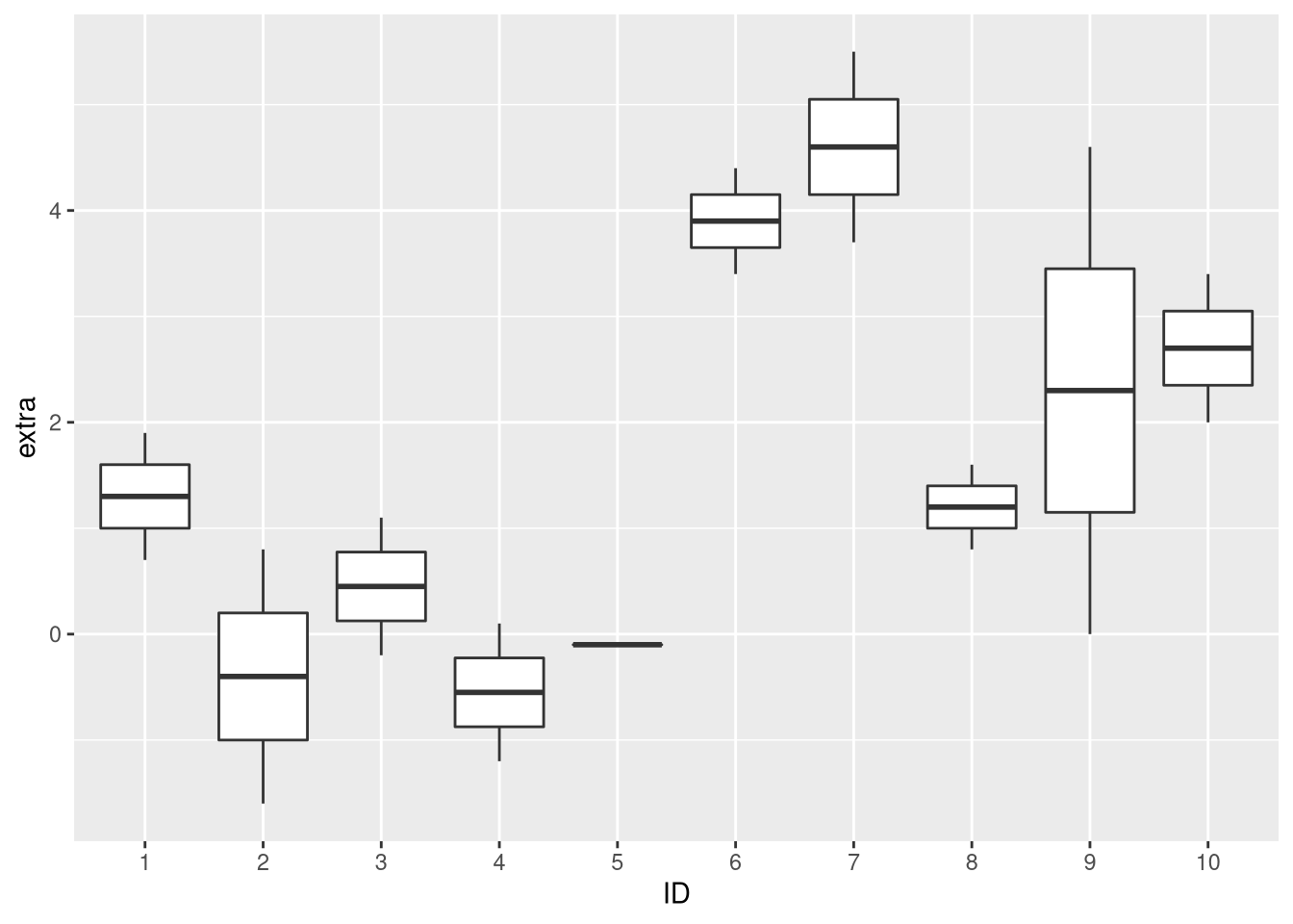

Indeed, the distribution of extra sleep time for the individual study subjects seems bimodal. About one half of the subjects exhibits large increases in sleep duration for both drugs, while the other half exhibits little benefit or even suffers from the medication. Using a paired test, these inter-patient differences can be corrected for, while this is not possible with a test that assumes that the measurements are independent.

Wilcoxon rank-sum test

If we use the unpaired Wilcoxon rank-sum test (Mann-Whitney U test) on the measurements, the test would generate the following order of drugs to determine significance:

# order sleep data by 'extra':
o <- order(sleep$extra)
# order drugs by increasing extra sleep time:
drug.order <- sleep$drug[o]
print(drug.order)

##  [1] 1 1 1 1 2 1 2 1 1 2 2 2 2 1 1 2 1 2 2 2
## Levels: 1 2

As we can see, although underrepresented, drug 1 occurs several times in the top ranks. This is because, for those patients that responded well to both drugs, drug 1 also worked well. Since there is no clear separation in the extra sleep time in dependence on the drug, the test fails to become significant at the 5% level:

x <- sleep$extra[sleep$drug == 1]
y <- sleep$extra[sleep$drug == 2]
# use an unpaired test:
w.unpaired <- wilcox.test(x, y, paired = FALSE)
print(w.unpaired$p.value)

## [1] 0.06932758

Wilcoxon signed rank test

Considering the measurements as pairs is more meaningful because then the result of the test is not influenced by the drug susceptibility in individual subjects. We can see that when we compute the intra-patient extra sleep difference, the measure that is used for the unpaired Wilcoxon signed rank test:

# compute pairwise differences of extra sleep times for the drugs
diff <- x - y
print(diff)

##  [1] -1.2 -2.4 -1.3 -1.3  0.0 -1.0 -1.8 -0.8 -4.6 -1.4

The non-positive differences clearly demonstrate that drug 1 is inferior to drug 2 across all study subjects. Since the Wilcoxon signed rank test is based on these differences, it finds that there’s a significant difference between the two drugs at a significance level of 5%:

# use a paired test:
w.unpaired <- wilcox.test(x, y, paired = TRUE)
print(w.unpaired$p.value)

## [1] 0.009090698