Comparing Measurements Across Several Groups: ANOVA
Parametric testing with the one-way ANOVA test
ANOVA stands for analysis of variance and indicates that test analyzes the within-group and between-group variance to determine whether there is a difference in group means.
The ANOVA test has three assumptions:
- The quantitative measurements are independent
- The ANOVA residuals are normally distributed
- The variance of the group measurements should be homogeneous (homoscedastic)
The most important assumption of ANOVA is the assumption of homoscedasticity, which should always be checked.
The InsectSprays data set
The InsectSprays data set compares the number of insects in agricultural units in which 6 different insect sprays were used. The data set has only two features: count indicates the insect count, while spray is a categorical variable indicating the used insect spray. For each of the insect sprays, the insect count was determined for 12 agricultural units.
To show how the test statistic is computed, we’ll transform the data set from long to wide format. For this purpose, we’ll add an ID column to indicate which entries belong into one row (note that this pairing of measurements is arbitrary and not relevant for the test):
df <- cbind(InsectSprays, ID = 1:12)
library(reshape2)
df <- dcast(df, ID ~ spray, value.var = "count")
df <- df[,-1] # remove ID column
print(df)
## A B C D E F
## 1 10 11 0 3 3 11
## 2 7 17 1 5 5 9
## 3 20 21 7 12 3 15
## 4 14 11 2 6 5 22
## 5 14 16 3 4 3 15
## 6 12 14 1 3 6 16
## 7 10 17 2 5 1 13
## 8 23 17 1 5 1 10
## 9 17 19 3 5 3 26
## 10 20 21 0 5 2 26
## 11 14 7 1 2 6 24
## 12 13 13 4 4 4 13The entries of df constitute a matrix \(X \in \mathbb{N}^{n \times p}\) with \(n\) rows and \(p\) columns (groups). The observation in row \(i\) and column \(j\) is denoted by \(x_{ij}\). The measurements for group \(i\) are indicated by \(X_i\), where \(\overline{X}_i\) indicates the mean of the measurements for group \(i\) and \(\overline{X}\) indicates the overall mean. Let \(n_j\) indicate the number of measurements for group \(j \in \{1, \ldots, p\}\). Note that the sample sizes do not have to be same
across groups for one-way ANOVA. This would only be a problem for factorial ANOVA (ANOVA with at least two independent variables) due to confounding.
Computing the ANOVA test statistic
The ANOVA test statistic is based on the between-group and the within-group mean-squared value.
Between-group mean-squared value
The sum of squared differences between the groups is:
\[SS_B = \sum_{j = 1}^p n_j(\overline{X}_j - \overline{X})\]
The value of \(SS_B\) indicates how much the group means deviate from the overall mean. To obtain the between-group mean-squared value, we divide by the between-group degrees of freedom, \(p-1\):
\[MS_B = \frac{SS_B}{p-1}\]
Within-group mean-squared value
The within-group sum of squares is defined as
\[SS_W = \sum_{j = 1}^p \sum_{i = 1}^{n_j} (x_{ij} - \overline{X}_j)^2\,.\]
The value of \(SS_W\) can be understood as the squared sum of the column entries after centering them using \(\overline{X}_j\). Its value indicates the variance of measurements within the groups. The within-group mean-squared value is obtained by dividing \(SS_W\) by the within-group degrees of freedom, \(\sum_{j=1}^p n_j - 1\):
\[MS_W = \frac{SS_W}{\sum_{j=1}^p n_j - 1}\]
The F-statistic
The F-statistic is the test statistic of the ANOVA test. It is defined as the ratio of the between-group and the within-group mean squared value:
\[F = \frac{MS_B}{MS_{W}}\]
The null hypothesis (groups have equal means) can be rejected if \(F\) is sufficiently large. In this case, \(MS_B\) is considerably larger than \(MS_W\). In this case, there are large differences between the means of the groups at a low variance within the groups.
Performing the ANOVA test in R
Before performing an ANOVA test, one should first confirm whether group variances are homogeneous. After running the test, it should be confirmed that the test residuals are normal.
Checking for homogeneous variance
To verify whether the variances are homogeneous across groups, we’ll generate a box plot of the insect counts:
data(InsectSprays)
library(ggplot2)
ggplot(InsectSprays, aes(x = spray, y = count)) + geom_boxplot() +
        xlab("Insect spray") + ylab("Insect count")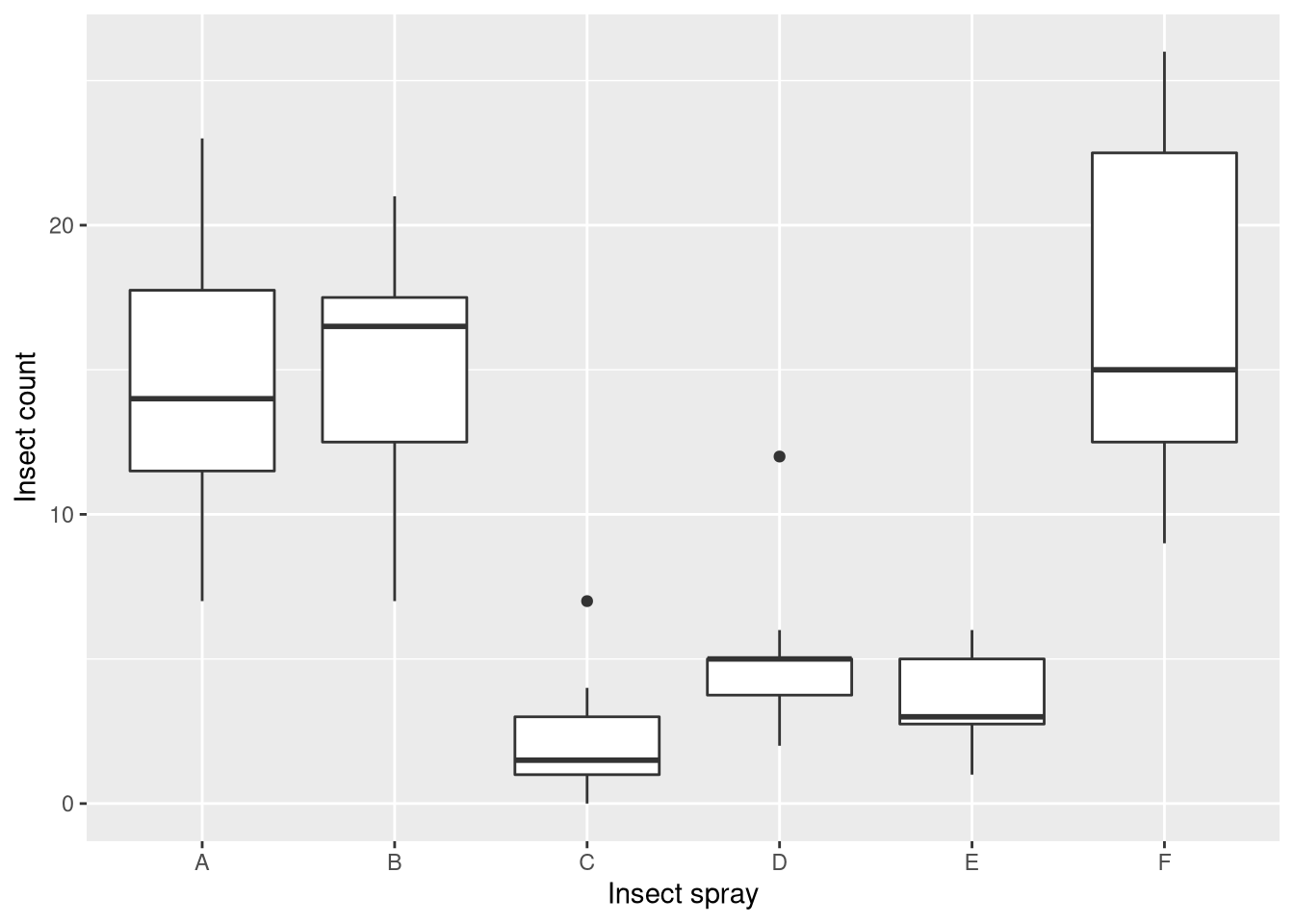
What we find is that sprays A, B, and F outperform sprays C, D, and E. Moreover the counts for A, B, and F have much higher variance than for the other sprays (the measurements are heteroscedastic). Thus, we will use the square-root transformation on the insect counts, which is a suitable variance-stabilizing transformation for count data. You can see the effect of the transformation here:
ggplot(InsectSprays, aes(x = spray, y = sqrt(count))) + geom_boxplot() +
        xlab("Insect spray") + ylab("Squared insect count")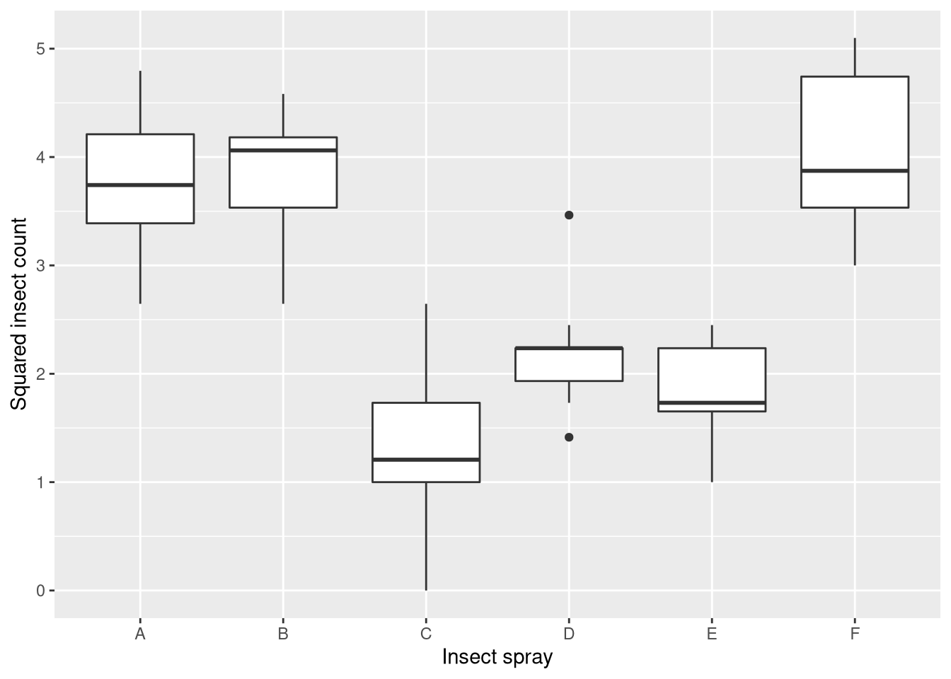
Running the ANOVA test
We can create the ANOVA model using the aov function by specifying a formula that indicates the variables and a corresponding data set:
# use sqrt to stabilize variance
spray.model <- aov(sqrt(count) ~ spray, data = InsectSprays)
Verifying whether residuals are normal
Based on spray.model, we can use the plot function to verify whether the residuals are normally distributed:
# check whether residuals are normally distributed:
plot(spray.model, which = 2)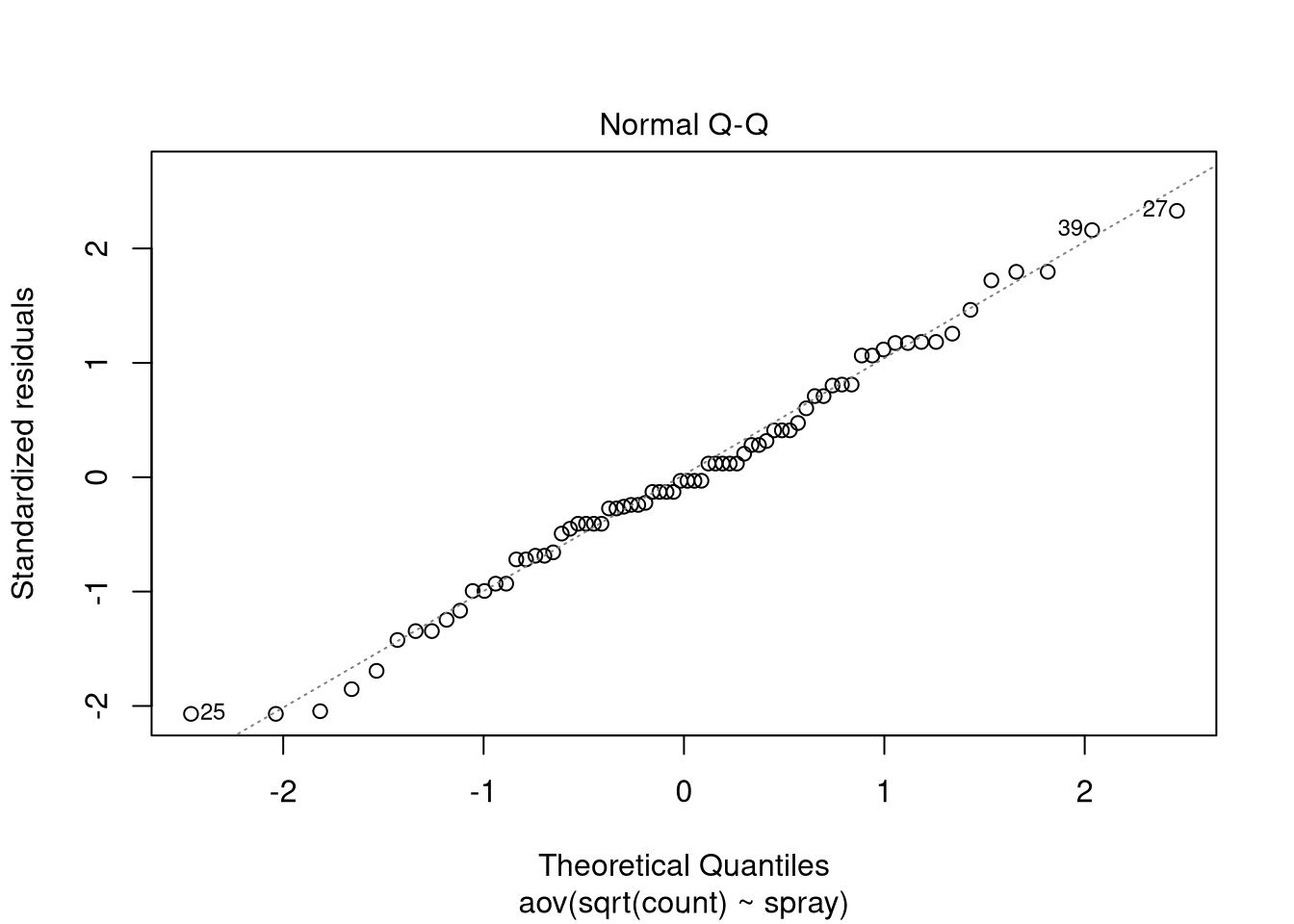
The linear trend in the measurements indicate that the residuals are normally distributed, so we can continue with retrieving the test results:
summary(spray.model)## Df Sum Sq Mean Sq F value Pr(>F)
## spray 5 88.44 17.688 44.8 <2e-16 ***
## Residuals 66 26.06 0.395
## ---
## Signif. codes: 0 '***' 0.001 '**' 0.01 '*' 0.05 '.' 0.1 ' ' 1The low p-value indicates that there is a significant different in the means of insect counts for different insect sprays.
Non-parametric testing with the Kruskal-Wallis test
If the assumptions of the ANOVA test do not hold, one can use a non-parametric ANOVA test, the Kruskal-Wallis test. In contrast to the parametric version of the test, Kruskal-Wallis test compares the medians of the groups rather than the means. Since the test is an extension of the Wilcoxon rank-sum test, their test statistics are computed in a similar manner. After ranking all observations, the test statistic can be obtained as:
\[H = (n − 1) \frac{\sum_{j = 1}^{p} n_j (\overline{r}_j - \overline{r})^2} {\sum_{j = 1}^p \sum_{i = 1}^{n_j} (r_{ij} − \overline{r})^2}\]
Here, \(\overline{r}_j = \frac{1}{n_j} \sum_{i = 1}^{n_j} r_{ij}\) is the average rank of all observations in group \(j\), \(r_ij\) is the rank of the \(i\)-th measurement in group \(j\), and \(\overline{r}\) is the average of all \(r_{ij}\). The interpretation of the test statistic is similar as for the parametric ANOVA: the enumerator indicates the between-group variance of ranks, which corresponds to the within-group sum of squared differences.
Applying the Kruskal-Wallis test in R
The Kruskal-Wallis test can be applied in the following way:
k.result <- kruskal.test(InsectSprays$count, InsectSprays$spray)
print(k.result)
##
## Kruskal-Wallis rank sum test
##
## data: InsectSprays$count and InsectSprays$spray
## Kruskal-Wallis chi-squared = 54.691, df = 5, p-value = 1.511e-10Again, the p-value indicates significance at a significance level of 5%. This time, however, the test result indicates that there is a difference in the median insect count across the groups rather than their means.
Summary
ANOVA is used to compare the mean/median of measurements across several groups. If you fulfill the assumptions of the parametric test, you can use the one-way ANOVA. Otherwise, you should use the non-parametric version of ANOVA, the Kruskal-Wallis test.


Comments
There aren't any comments yet. Be the first to comment!