Mean vs Median: When to Use Which Measure?
The mean
The arithmetic mean is what most people simply know as the average. To be exact, however, we have to note that the mean is just one type of average. Before getting lost in the intricacies of these terms, let’s move on to the definition of the mean
Given a vector \(x\) with \(n\) entries, the mean is defined as
\[\overline{x} = \frac{1}{n} \sum_{i = 1}^n x_i\]
Assume we have \(x = (30, 25, 40, 41, 30, 41, 50, 33, 40, 1000)\), what would be the mean? We can compute it in the following ways:
x <- c(30, 25, 40, 41, 30, 41, 50, 33, 40, 1000)
# the way of the beginner (don't do this!):
x.mean <- 0
for (xi in x) {
    x.mean <- x.mean + xi
}
x.mean <- x.mean / length(x)
print(x.mean)
## [1] 133# a better way:
x.mean <- sum(x) / length(x)
print(x.mean)## [1] 133# the right way:
x.mean <- mean(x)
print(x.mean)## [1] 133As you can see, you can simply use the mean function rather than having to implement the mean by yourself.
The median
The median refers to the most central value in a list of numbers. While simple to explain, the median is harder to compute than the mean. This is because in order to find the median, it is necessary to sort the numbers in the list. Moreover, we have to differentiate two cases. If the list has an odd number of elements, then the median is the most central member in the list. However, if the list has an even number of elements, we need to determine the arithmetic mean of the two most central numbers.
We can formalize this in the following way. Let \(x\) be a sorted vector of numbers. Then the median is
\[\text{median}(x) = \begin{cases} x_{1 + \lfloor n/2 \rfloor} & \text {if $n$ is odd} \\ \frac{1}{2} \cdot (x_{n/2} + x_{1 + n/2}) & \text {if $n$ is even} \\ \end{cases} \]
where \(\lfloor . \rfloor\) is the floor function.
Let’s see how we can obtain the median in R.
# the hard way (don't do it like that)
mymedian <- function(x) {
    x <- sort(x)
    n <- length(x)
    median <- NULL
    if (n %% 2 == 0) {
        # length is even
        median <- mean(c(x[n/2], x[n/2 + 1]))
    } else {
        # length is odd
        median <- x[floor(n/2)]
    }
    return(median)
}
x.median <- mymedian(x)
print(x.median)
## [1] 40# the easy way:
x.median <- median(x)
print(x.median)## [1] 40Comparison of mean and median
Having defined both types of averages, we can now look into the difference between the two. While the arithmetic mean considers all the values in a vector, the median value only considers a subset of values. This is because the median basically discards all vector elements except for the most central value(s). This feature of the median can make a big difference. As we have seen in our example, the mean of \(x\) (133) was much larger than its median (40). In this case, this is because the median discards the value 1000 in \(x\), while the arithmetic mean considers it.
This brings us to the question we wanted to answer: when to use the mean and when to use the median? The answer is simple. If your data contains outliers such as the 1000 in our example, then you would typically rather use the median because otherwise the value of the mean would be dominated by the outliers rather than the typical values. In conclusion, if you are considering the mean, check your data for outliers. A simple way to do this is to plot a histogram of the data.
hist(x)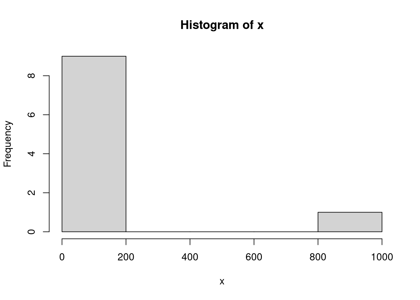
For our data, the histogram clearly shows the outlier with a value of 1000 and we conclude that the median would be more appropriate than the mean.
Can you think of other situations when you would rather use the median than the mean? Let me know in the comments!


Comments
Omar
06 Sep 20 21:25 UTC