Type 1 vs Type 2 Errors: Significance vs Power
Type 1 vs type 2 error
Type 1 and type 2 errors are defined in the following way for a null hypothesis \(H_0\):
| Decision/Truth | \(H_0\) true | \(H_0\) false |
|---|---|---|
| \(H_0\) rejected | Type 1 error (\(\alpha\)) | Correctly rejected (Power, \(1-\beta\)) |
| Failed to reject \(H_0\) | Correctly not rejected | Type 2 error (\(\beta\)) |
Type 1 and type 2 error rates are denoted by \(\alpha\) and \(\beta\), respectively. The power of a statistical test is defined by \(1 - \beta\). In summary:
- The significance level answers the following question: If there is no effect, what is the likelihood of falsely detecting an effect? Thus, significance is a measure of specificity.
- The power answers the following question: If there is an effect, what is the likelihood of detecting it? Thus, power is a measure of sensitivity.
The power of a test depends on the following factors:
- Effect size: power increases with increasing effect sizes
- Sample size: power increases with increasing number of samples
- Significance level: power increases with increasing significance levels
- The test itself: some tests have greater power than others for a given data set
Traditionally, the type 1 error rate is limited using a significance level of 5%. Experiments are often designed for a power of 80% using power analysis. Note that it depends on the test whether it’s possible to determine the statistical power. For example, power is determined more readily available for parametric than for non-parametric tests.
Choice of the null hypothesis
Since the type 1 error rate is typically more stringently controlled than the type 2 error rate (i.e. \(\alpha < \beta\)), the alternative hypothesis often corresponds to the effect you would like to demonstrate. In this way, if the null hypothesis is rejected, it is unlikely that the rejection is a type 1 error. When statistical testing is used to inform decision making, the null hypothesis whose type 1 error would have the worse consequence should be selected. Let’s consider two examples for choosing the null hypothesis in this manner.
Example 1: introduction of a new drug
Let’s assume there’s a well-tried, FDA-approved drug that is effective against cancer. Having developed a new drug, your company wants to decide whether it should supplant the old drug with the new drug. Here, you definitely want to use a directional test in order to show that one drug is superior over the other. However, given effectivity measures A and B for the old and the new drug, respectively, how should the null hypothesis be formulated? Take a look at the consequences of the choice:
| Null hypothesis | Type 1 error | Impact of type 1 error |
|---|---|---|
| \(A \geq B\) | Incorrectly reject \(A \geq B\) | You falsely conclude that drug B is superior to drug A. Thus, you introduce B to the market, thereby risking the life of patients where B was favored over A. |
| \(A \leq B\) | Incorrectly reject \(A \leq B\) | You falsely conclude that drug A is superior to drug B. Thus, albeit actually superior to A, B is never released and resources have been wasted. |
Evidently, having \(H_0: A \geq B\) is the more appropriate null hypothesis because its type 1 error is more detrimental (lives are endangered) than that of the other null hypothesis (patients do not receive access to a better drug).
Example 2: change in taxation
The government thinks about simplifying the taxation system. Let A be the amount of tax income with the old, complicated system and let B be the income with the new, simplified system.
| Null hypothesis | Type 1 error | Impact of type 1 error |
|---|---|---|
| \(A \geq B\) | Incorrectly reject \(A \geq B\) | Incorrectly conclude that the new system leads to greater income. So, after changing to the simplified taxation system, you realize that you actually acquire fewer taxes. |
| \(A \leq B\) | Incorrectly reject \(A \leq B\) | Incorrectly conclude that the old system was better. You don’t introduce the simplified approach and miss out on additional taxation income. |
In this case, assuming that the new system leads to less income from taxation, that is, \(H_0: A \geq B\) is clearly the better option (if you are optimizing with regard to tax income). In this case, a type 1 error means that the taxation system doesn’t have to be changed. Using the other null hypothesis, a type 1 error would mean that the system would have to be changed (this is costly!) and that the state would receive fewer income from taxes.
The two examples suggest the following motto for significance testing: Never change a running system. When comparing a new system with a well-tried system, always set the null hypothesis to the assumption that the new system is worse than the old one. Then, if the null hypothesis is rejected, we can be quite sure that it’s worth to replace the old system with the new one because a type 1 error is unlikely.
How to select the significance level?
Typically the significance level is set to 5%. If you are thinking about lowering the significance level, you should make sure that the test you are about to perform has sufficient statistical power. Particularly for small sample sizes, lowering the significance level can critically increase the type 2 error.
Assume we want to use a t-test on the null hypothesis that drug B has less or equal mean effectivity than drug A. Then we can use the power.t.test function from the pwr package. Assume that drug B exhibits a mean increase in effectivity larger than 0.5 (delta parameter) and that the standard deviation of the measurements is 1. Since we really want to avoid type 1 errors here, we require a low significance level of 1% (sig.level parameter). Let’s see how power changes with the sample size:
library(pwr)
sample.size <- c(10,20,30, 40, 50, 75, 100, 125, 150, 175, 200)
power <- rep(NA, length(sample.size))
for (i in seq_along(sample.size)) {
    n <- sample.size[i]
    t <- power.t.test(n = n, delta = 0.5, sd = 1,
                      sig.level = 0.01, alternative = "one.sided")
    power[i] <- t$power
}
power.df <- data.frame("N" = sample.size, "Power" = power)
library(ggplot2)
ggplot(power.df, aes(x = N, y = Power)) + geom_point() + geom_line()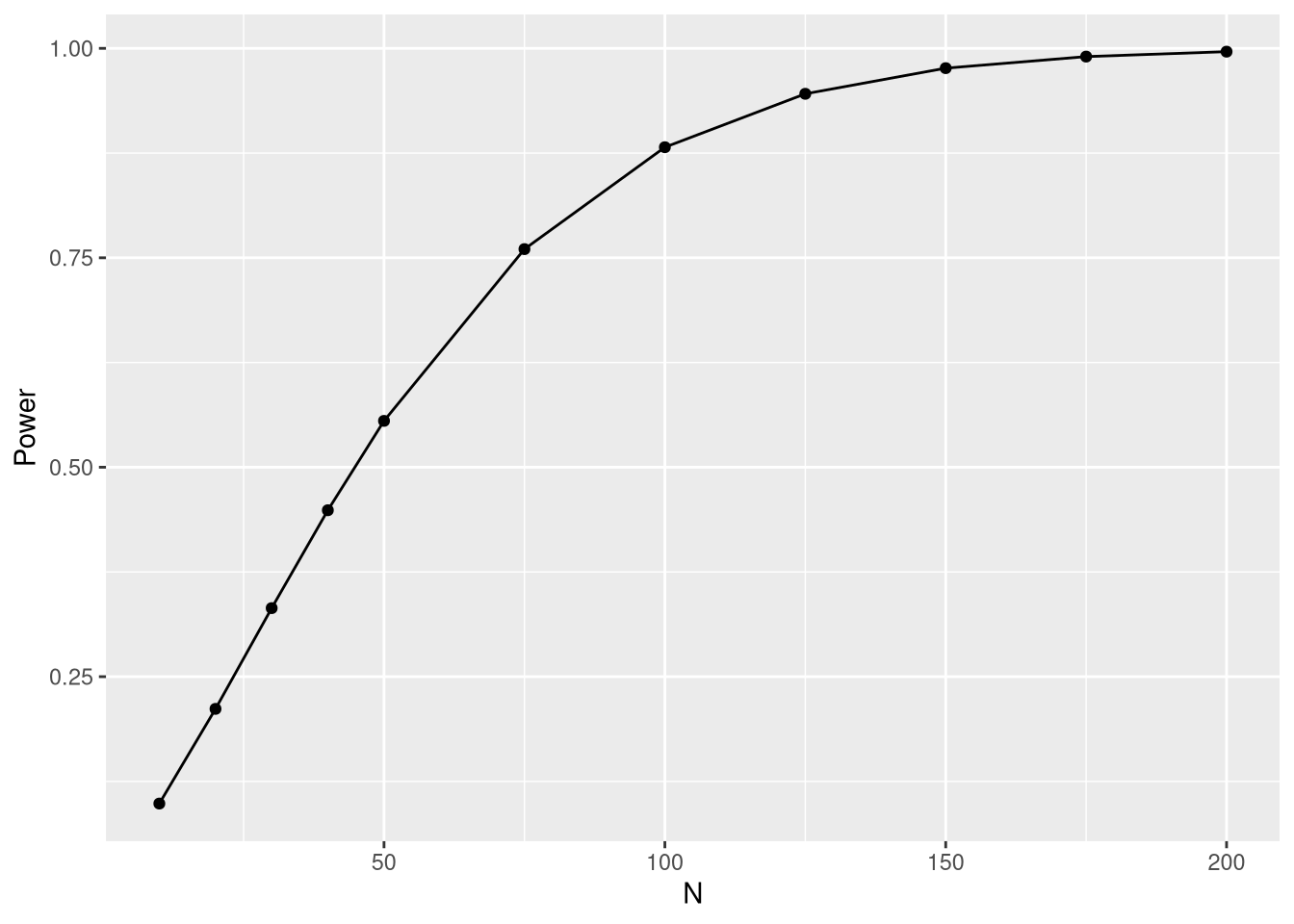
What do the results mean? For only 50 measurements per group and a 1% significance level, the power would merely be 55.5%. So, if B were actually better than A, we would fail to reject the null hypothesis in 44.5% of cases. This type 2 error rate is way too high and thus a significance level of 1% should not be selected. On the other hand, with 150 samples per group we wouldn’t have any problems because we would have a type 2 error rate of 2.4% at the 1% significance level.
So, what should we do if the sample size is only 50 per group? In this case, we would be inclined to use a less stringent significance level. How lenient should it be? We can find out by requiring a power of 80%:
t <- power.t.test(n = 50, delta = 0.5, sd = 1, power = 0.8,
                  sig.level = NULL, alternative = "one.sided")
print(t$sig.level)
## [1] 0.05038546Thus, for 50 samples per group, adequate power would be obtained if the significance level is set to 5%.


Comments
There aren't any comments yet. Be the first to comment!