Navigating in Gridworld using Policy and Value Iteration
Learn how to use policy evaluation, policy iteration, and value iteration to find the shortest path in gridworld.
In reinforcement learning, we are interested in identifying a policy that maximizes the obtained reward. Assuming a perfect model of the environment as a Markov decision process (MDPs), we can apply dynamic programming methods to solve reinforcement learning problems.
In this post, I present three dynamic programming algorithms that can be used in the context of MDPs. To make these concepts more understandable, I implemented the algorithms in the context of a gridworld, which is a popular example for demonstrating reinforcement learning.
Before we being with the application, I would like to quickly provide the theoretical background that is required for the following work on the gridworld.
Key Reinforcement Learning Terms for MDPs
The following sections explain the key terms of reinforcement learning, namely:
- Policy: Which actions the agent should execute in which state
- State-value function: The expected value of each state with regard to future rewards
- Action-value function: The expected value of performing a specific action in a specific state with regard to future rewards
- Transition probability: The probability to transition from one state to another
- Reward function: The reward that the agent obtains when transitioning between states
Policy
A policy, \(\pi(s,a)\), determines the probability of executing action \(a\) in state \(s\). In deterministic environments, a policy directly maps from states to actions.
State-Value Function
Given a policy \(\pi\), the state-value function \(V^{\pi}(s)\) maps each state \(s\) to the expected return that the agent can obtain in this state:
\[V^{\pi}(s) = E_{\pi} \{R_t | s_t = s\} = E_{\pi} \{\sum_{k=0}^{\infty} \gamma^k r_{t+k+1} | s_t = s\}\]
In the formula, \(s_t\) indicates the state at time \(t\). The parameter \(\gamma \in [0,1]\) is called the discount factor. It determines the impact of rewards in the future. If we set \(\gamma = 1\), this indicates that we are sure about the future because we do not have to discount future rewards. For \(\gamma < 1\), we take the uncertainty about the future into account and give greater weight to more recently earned rewards.
Action-Value Function
Given a policy \(\pi\), the action-value function \(Q{^\pi}(s,a)\) determines the expected reward when executing action \(a\) in state \(s\):
\[Q^{\pi}(s,a) = E_{\pi}\{R_t | s_t = s, a_t = a\} = E_{\pi} \{\sum_{k=0}^{\infty} \gamma^k r_{t+k+1} | s_t = s, a_t = a\} \]
Transition Probability
Executing an action \(a\) in state \(s\) may transition the agent to state \(s'\). The probability that this transition takes place is described by \(P_{ss'}^a\).
Reward Function
The reward function, \(R_{ss'}^a\), specifies the reward that is obtained when the agent transitions from state \(s\) to state \(s'\) via action \(a\).
Demonstration of Three Basic MDP Algorithms in Gridworld
In this post, you will learn how to apply three algorithms for MDPs in a gridworld:
- Policy Evaluation: Given a policy \(\pi\), what is the value function associated with \(\pi\)?
- Policy Iteration: Given a policy \(\pi\), how can we find the optimal policy \(\pi^{\ast}\)?
- Value Iteration: How can we find an optimal policy \(\pi^{\ast}\) from scratch?
In gridworld, the goal of the agent is to reach a specified location in the grid. The agent can either go north, go east, go south, or go west. These actions are represented by the set : \(\{N, E, S, W\}\). Note that the agent knows the state (i.e. its location in the grid) at all times.
To make life a bit harder, there are walls in the grid through which the agent cannot pass. Rather, when trying to move through a wall, the agent remains in its position. For example, when the agent chooses action \(N\) and there is a wall to the north of the agent, the agent will remain in its place.
Basic Gridworld Implementation
I’ve implemented the gridworld in an object-oriented manner. The following sections describe how I designed the code for the map and the policy entities.
Representing the Gridworld Map
To implement gridworld, the first thing I started with was a class for representing the map. I defined the following format to represent individual grid cells:
#indicate wallsXindicates the goal- Blanks indicate empty tiles
Relying on these symbols, I constructed the following map, which is used in the following work:
###################
#                X#
#   ###########   #
#   #         #   #
#   # ####### #   #
#   # #     # #   #
#     #  #  #     #
#        #        #
#                 #
###             ###
#                 #
###################
The map-related entities of the code are structured like this:

I implemented MapParser, which generates a Map object. The map object controls the access to the cells of the gridworld. Individual cell subclasses define the behavior of specific cells such as empty cells, walls, and the goal cell. Each cell can be identified using its row and column index.
With this setup, a map can be conveniently loaded:
parser = MapParser()
gridMap = parser.parseMap("../data/map01.grid")
Loading a Policy
For reinforcement learning, we need to be able to deal with a policy, \(\pi(s,a)\). In gridworld, each state \(s\) represents a position of the agent. The actions move the agent one step into one of the four geographic directions. We will use the following symbols to map a policy onto a map:
- N for the action
GO_NORTH - E for the action
GO_EAST - S for the action
GO_SOUTH - W for the action
GO_WEST
Unknown symbols are mapped to a NONE action in order to obtain a complete policy.
Using these definitions, I defined the following policy:
###################
#EESWWWWWWWWWWWWWX#
#EES###########SWN#
#EES#EEEEEEEES#SWN#
#EES#N#######S#SWN#
#EES#N#SSWWW#S#SWN#
#EEEEN#SS#NN#SWSWN#
#EENSSSSS#NNWWWWWN#
#EENWWWWEEEEEEEEEN#
###NNNNNNNNNNNNN###
#EENWWWWWWWWWWWWWW#
###################
Note that the policy file retains the walls and the goal cell for better readability. The policy was written with two goals in mind:
- The agent should be able to reach the goal. With a policy where this property is not fulfilled, policy evaluation will not give a reasonable result because the reward at the goal will never be earned.
- The policy should be suboptimal. This means that there are states where the agent doesn’t take the shortest path to the goal. Such a policy allows us to see the effect of algorithms that try to improve upon the initial policy.
To load the policy, I implemented a policy parser, which stores the policy as a policy object. Using these objects, we can load our initial policy like so:
policyParser = PolicyParser()
policy = policyParser.parsePolicy("../data/map01.policy")
The policy object has a function for modeling \(\pi(s,a)\):
def pi(self, cell, action):
    if len(self.policy) == 0:
        # no policy: try all actions (for value iteration)
        return 1

    if self.policyActionForCell(cell) == action:
        # policy allows this action
        return  1
    else:
        # policy forbids this action
        return 0
Preparations for Reinforcement Learning
To prepare the implementation of the reinforcement learning algorithms, we still need to provide a transition and a reward function.
Transition Function
To define the transition function \(P_{ss'}^a\), we first need to to differentiate between illegal and legal actions. In gridworld, there are two ways that an action can be illegal:
- If the action would take the agent off the grid
- If the action would move the agent into a wall
The gives us the first rule for the transition function:
1. When an action is illegal, the agent should remain in its previous state.Additionally, we must also require:
2. When an action is illegal, transitions to states other than its previous state should be forbidden.So what about legal actions? Of course, state transition must be valid with regard to the chosen action. Since each action moves the agent only a single position, a proposed state \(s'\) must have the agent in a cell that is adjacent to the one in state \(s\):
3. Only allow transitions through actions that would lead the agent to an adjacent cell.For this rule, we assume that there is a predicate \(adj(s,s')\) to indicate whether the agent’s transition from \(s\) to \(s'\) involved adjacent cells.
Finally, once we have reached the goal state, \(s^{\ast}\), we don’t want the agent to move away again. To stipulate this, we introduce the final rule:
4. Don't transition from the goal cell.Based on these four rules, we can define the transition function as follows:
\[P_{ss'}^a = \begin{cases} 1 & \forall \quad \text{illegal action with $s = s'$} & \text{Rule 1} \\ 0 & \forall \quad \text{illegal action with $s \neq s'$} &\text{Rule 2} \\ 1 & \forall \quad \text{legal action with adj(s,s')} & \text{Rule 3} \\ 0 & \forall \quad \text{if $s = s^{\ast}$} & \text{Rule 4} \end{cases} \]
The Python implementation provided by getTransitionProbability is a not as clear-cut as the mathematical formulation, but I will provide it nonetheless:
def transitionProbabilityForIllegalMoves(oldState, newState):
    if newState == oldState:
        # Rule 1: stay at oldState if action is illegal
        return 1
    else:
        # Rule 2: dont transition to 'newState' if action is illegal
        return 0

def getTransitionProbability(self, oldState, newState, action, gridWorld):
    proposedCell = gridWorld.proposeMove(action)
    if proposedCell is None:
        # Rule 1 and 2: illegal move
        return transitionProbabilityForIllegalMoves(oldState, newState)
    if oldState.isGoal():
        # Rule 4: stay at goal
        return 0
    if proposedCell != newState:
        # Rule 3: move not possible
        return 0
    else:
        # Rule 3: move possible
        return 1
Note that proposeMove simulates the successful execution of an action and returns the new grid cell of the agent.
Reward Function
In gridworld, we want to find the shortest path to the terminal state. We want to maximize the obtained rewards, so the reward at the goal state, \(s^{\ast}\) should be higher than the reward at the other states. For the gridworld, we will use the following simple function:
\[R_{ss'}^a = \begin{cases} -1 & \forall s' \neq s^{\ast} \\ 0 & \forall s' = s^{\ast} \end{cases} \]
The Python implementation is given by
def R(self, oldState, newState, action):
        # reward for state transition from oldState to newState via action
        if newState and newState.isGoal():
            return 0
        else:
            return -1
Policy Evaluation
The goal of the policy evaluation algorithm is to evaluate a policy \(\pi(s,a)\), that is, to determine the value of all states in terms of \(V(s) \forall s\). The algorithm is based on the Bellman equation: \[V_{k+1}(s) = \sum_{a} \pi(s,a) \sum_{s'} P_{ss'}^a [R_{ss'}^a + \gamma V^{\pi}_k(s')] \] For iteration \(k+1\), the equation yields the value of state \(s\) via:
- \(\pi(s,a)\): the probability of choosing action \(a\) in state \(s\)
- \(P_{ss'}^a\): the probability of transitioning from state \(s\) to state \(s'\) using action \(a\)
- \(R_{ss'}^a\): the expected reward when transitioning from state \(s\) to state \(s'\) using action \(a\)
- \(\gamma\): the discount rate
- \(V^{\pi}_k(s')\): the value of state \(s'\) in step \(k\), given the policy \(\pi\)
For a better understanding of the equations, let’s consider it piece by piece, in the context of gridworld:
- \(\pi(s,a)\): Since we’re in a deterministic environment, a policy only specifies a single action, \(a\), with \(\pi(s,a) = 1\), while all other actions, \(a'\), have \(\pi(s,a') = 0\). So, the multiplication by \(\pi(s,a)\) just selects the action that is specified by the policy.
- \(\sum_{s'}\): This sum is over all states, \(s'\), that can be reached from the current state \(s\). In gridworld, we merely need to consider adjacent cells and the current cell itself, i.e. \(s' \in \{x | adj(x,s) \lor x = s\}\).
- \(P_{ss'}^a\): This is the probability of transitioning from state \(s\) to \(s'\) via action \(a\).
- \(R_{ss'}^a\): This is the reward for the transition from \(s\) to \(s'\) via \(a\). Note that in gridworld, the reward is merely determined by the next state, \(s'\).
- \(\gamma\): The discounting factor modulates the impact of the expected reward.
- \(V_{k}(s')\): The expected reward at the proposed state, \(s'\). The presence of this term is why policy evaluation is dynamic programming: we are using previously computed values to update the current value.
We will use \(\gamma = 1\) because we are in an episodic setting where learning episodes stop when we reach the goal state. Because of this, the value function represents the length of the shortest path to the goal cell. More, precisely, let \(d(s,s^{\ast})\) indicate the shortest path from state \(s\) to the goal. Then, \(V^{\pi}(s) = -d(s, s^{\ast}) + 1\) for \(s \neq s^{\ast}\).
To implement policy evaluation, we will typically perform multiple sweeps of the state space. Each sweep requires the value function from the previous iteration. The difference between the new and old value function is often used as a stopping criterion for the algorithm:
def findConvergedCells(self, V_old, V_new, theta = 0.01):
    diff = abs(V_old-V_new)
    return np.where(diff < theta)[0]
The function determines the indices of grid cells whose value function difference was less than \(\theta\). When the values of all states have converged to a stable value, we can stop. Since this is not always the case (e.g. if the policy specifies states with actions that do not lead to the goal or when the transition probabilities/rewards are configured inappropriately), we also specify a maximal number of iterations.
Once the stopping criterion is reached, evaluatePolicy returns the latest state-value function:
def evaluatePolicy(self, gridWorld, gamma = 1):
    if len(self.policy) != len(gridWorld.getCells()):
        # sanity check whether policy matches dimension of gridWorld
        raise Exception("Policy dimension doesn't fit gridworld dimension.")
    maxIterations = 500
    V_old = None
    V_new = initValues(gridWorld) # sets value of 0 for viable cells
    iter = 0
    convergedCellIndices = np.zeros(0)
    while len(ConvergedCellIndices) != len(V_new):
        V_old = V_new
        iter += 1
        V_new = self.evaluatePolicySweep(gridWorld, V_old, gamma, convergedCellIndices)
        convergedCellIndices = self.findConvergedCells(V_old, V_new)
        if iter > maxIterations:
            break
    print("Policy evaluation converged after iteration: " + str(iter))
    return V_new
Once sweep of policy evaluation is performed by the evaluatePolicySweep function. The function iterates over all cells in the grid and determines the new value of the state:
def evaluatePolicySweep(self, gridWorld, V_old, gamma, ignoreCellIndices):
    V = initValues(gridWorld)
    # evaluate policy for every state (i.e. for every viable actor position)
    for (i,cell) in enumerate(gridWorld.getCells()):
        if np.any(ignoreCellIndices == i):
            V[i] = V_old[i]
        else:
            if cell.canBeEntered():
                gridWorld.setActor(cell)
                V_s = self.evaluatePolicyForState(gridWorld, V_old, gamma)
                gridWorld.unsetActor(cell)
                V[i] = V_s
    self.setValues(V)
    return V
Note that the ignoreCellIndices parameter represents the indices of cells for which subsequent sweeps didn’t change the value function. These cells are ignored in further iterations to improve the performance. This is fine for our gridworld example because we are just interested in finding the shortest path. So, the first time that a state’s value function doesn’t change, this is its optimal value.
The value of a state is computed using the evaluatePolicyForState function. At its core, the function implements the equations from Bellman that we talked about earlier. An important idea for this function is that we do not want to scan all states \(s'\) when computing the value function for state \(s\). This is why the state generator generates only those states that can actually occur (i.e. have a transition probability greater than zero).
def evaluatePolicyForState(self, gridWorld, V_old, gamma):
    V = 0
    cell = gridWorld.getActorCell()
    stateGen = StateGenerator()
    transitionRewards = [-np.inf] * len(Actions)
    for (i, actionType) in enumerate(Actions):
        gridWorld.setActor(cell) # set state
        actionProb = self.pi(cell, actionType)
        if actionProb == 0 or actionType == Actions.NONE:
            continue
        newStates = stateGen.generateState(gridWorld, actionType, cell)
        transitionReward = 0
        for newActorCell in newStates:
            V_newState = V_old[newActorCell.getIndex()]
            # Bellman equation
            newStateReward = getTransitionProbability(cell, newActorCell, actionType, gridWorld) *\
                                (R(cell, newActorCell, actionType) +\
                                gamma * V_newState)
            transitionReward += newStateReward
        transitionRewards[i] = transitionReward
        V_a = actionProb * transitionReward
        V += V_a
    if len(self.policy) == 0:
        V = max(transitionRewards)
    return V
Results from Policy Evaluation
With the implementation in place, we can find the state-value function of our policy by executing:
V = policy.evaluatePolicy(gridMap)To draw the value function together with the policy, we can use pyplot from matplotlib after converting the 1-D array that is used to represent the map to a 2D-array:
def drawValueFunction(V, gridWorld, policy):
    fig, ax = plt.subplots()
    im = ax.imshow(np.reshape(V, (-1, gridWorld.getWidth())))
    for cell in gridWorld.getCells():
        p = cell.getCoords()
        i = cell.getIndex()
        if not cell.isGoal():
            text = ax.text(p[1], p[0], str(policy[i]),
                       ha="center", va="center", color="w")
        if cell.isGoal():
            text = ax.text(p[1], p[0], "X",
                       ha="center", va="center", color="w")
    plt.show()
Using the function, we can visualize the state-value function of our policy:
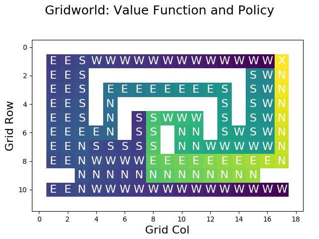
For non-goal cells, the plot is annotated with the actions specified by the policy. The goal in the upmost right cell is indicated by the X label. Walls (infinite value) are shown in white.
The value of the others cells is indicated by color. The worst states (with the lowest reward) are shown in purple, bad states in blue, intermediate states in turquois, good states in green, and very good states (with the highest reward) are shown in yellow.
Looking at the values, we can see that the results match the actions that are dictated by the policy. For example, the state directly to the west of the goal has a very low value because this state’s action (GO_WEST) leads to a long detour. The cell directly south of the goal has a very high value because its action (GO_NORTH) leads directly to the goal.
Note that, for our future work, the performance of evaluatePolicy is of critical concern because we will call it many times. For the computed example, the function requires 61 iterations, which translates to roughly half a second on my laptop. Note that the policy evaluation will require fewer iterations for policies that are closer to the optimal policy because values will propagate faster.
Being able to determine the state-value function is nice - now we can quantify the merit of a proposed policy is. However, we haven’t yet dealt with the problem of finding an optimal policy. This is where policy iteration comes into play.
Policy Iteration
Now that we are able to compute the state-value function, we should be able to improve an existing policy. A simple strategy for this is a greedy algorithm that iterates over all the cells in the grid and then chooses the action that maximizes the expected reward according to the value function.
This approach implicitly determines the action-value function, which is defined as
\[Q^{\pi}(s,a) = \sum_{s'} P_{ss'}^a [R_{ss'}^a + \gamma V^{\pi}(s')] \]
The improvePolicy function determines the value function of a policy (if it’s not available yet) and then calls findGreedyPolicy to identify the optimal action for every state:
def improvePolicy(policy, gridWorld, gamma = 1):
    policy = copy.deepcopy(policy) # dont modify old policy
    if len(policy.values) == 0:
        # policy needs to be evaluated first
        policy.evaluatePolicy(gridWorld)
    greedyPolicy = findGreedyPolicy(policy.getValues(), gridWorld, \
                    policy.gameLogic, gamma)
    policy.setPolicy(greedyPolicy)
    return policy

def findGreedyPolicy(values, gridWorld, gameLogic, gamma = 1):
    # create a greedy policy based on the values param
    stateGen = StateGenerator()
    greedyPolicy = [Action(Actions.NONE)] * len(values)
    for (i, cell) in enumerate(gridWorld.getCells()):
        gridWorld.setActor(cell)
        if not cell.canBeEntered():
            continue
        maxPair = (Actions.NONE, -np.inf)
        for actionType in Actions:
            if actionType == Actions.NONE:
                continue
            proposedCell = gridWorld.proposeMove(actionType)
            if proposedCell is None:
                # action is nonsensical in this state
                continue
            Q = 0.0 # action-value function
            proposedStates = stateGen.generateState(gridWorld, actionType, cell)
            for proposedState in proposedStates:
                actorPos = proposedState.getIndex()
                transitionProb = gameLogic.getTransitionProbability(cell, proposedState, actionType, gridWorld)
                reward = gameLogic.R(cell, proposedState, actionType)
                expectedValue = transitionProb * (reward + gamma * values[actorPos])
                Q += expectedValue
            if Q > maxPair[1]:
                maxPair = (actionType, Q)
        gridWorld.unsetActor(cell) # reset state
        greedyPolicy[i] = Action(maxPair[0])
    return greedyPolicy
What findGreedyPolicy does is to consider each cell and to select that action maximizing its expected reward, thereby constructing an improved version of the input policy. For example, after executing improvePolicy once and re-evaluating the policy, we obtain the following result:
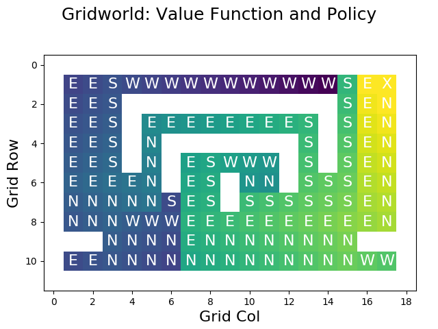
In comparison to the original value function, all cells next to the goal are giving us a high reward now because the actions have been optimized. However, we can see that these improvements are merely local. So, how can we obtain an optimal policy?
The idea of the policy iteration algorithm is that we can find the optimal policy by iteratively evaluating the state-value function of the new policy and to improve this policy using the greedy algorithm until we’ve reached the optimum:
def policyIteration(policy, gridWorld):
    lastPolicy = copy.deepcopy(policy)
    lastPolicy.resetValues() # reset values to force re-evaluation of policy
    improvedPolicy = None
    while True:
        improvedPolicy = improvePolicy(lastPolicy, gridWorld)
        if improvedPolicy == lastPolicy:
            break
        improvedPolicy.resetValues() # to force re-evaluation of values on next run
        lastPolicy = improvedPolicy
    return(improvedPolicy)
Results from Policy Iteration
Running the algorithm on the gridworld leads to the optimal solution within 20 iterations - about 4,5 seconds on my notebook. The termination after 20 iterations doesn’t come as a surprise: the width of the gridworld map is 19. So we need 19 iterations to optimize the values of the horizontal corridor. Then, we need one additional iteration to determine that the algorithm can terminate because the policy hasn’t changed.
A great tool for understanding policy iteration is by visualizing each iteration:
The following figure shows the optimal value function that has been constructed using policy iteration:
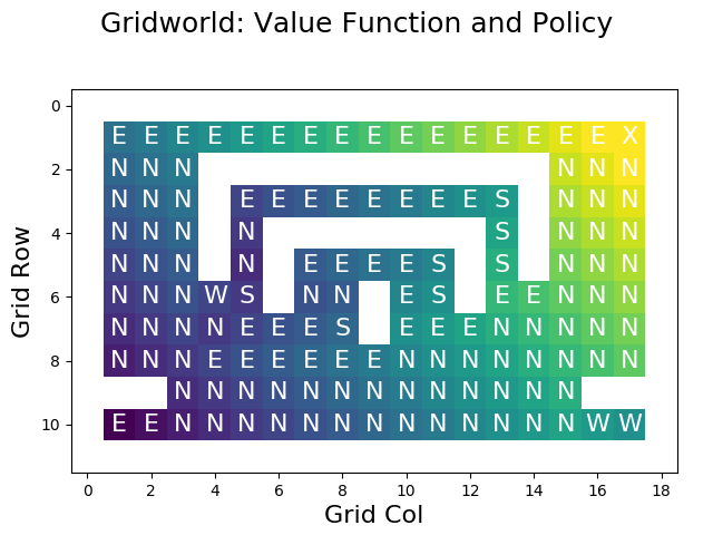
Visual inspection shows that the value function is correct, as it chooses the shortest path for each cell in the grid.
Value Iteration
With the tools we have explored until now, a new question arises: why do we need to consider an initial policy at all? The idea of the value iteration algorithm is that we can compute the value function without a policy. Instead of letting the policy, \(\pi\), dictate which actions are selected, we will select those actions that maximize the expected reward:
\[V_{k+1}(s) = \max_{a} \sum_{s'} P_{ss'}^a [R_{ss'}^a + \gamma V_k(s')] \]
Because the computations for value iteration are very similar to policy evaluation, I have already implemented the functionality for doing value iteration into the evaluatePolicyForState method that I defined earlier. I marked the relevant lines with >:
def evaluatePolicyForState(self, gridWorld, V_old, gamma):
    V = 0
    cell = gridWorld.getActorCell()
    stateGen = StateGenerator()
    transitionRewards = [-np.inf] * len(Actions)
    for (i, actionType) in enumerate(Actions):
        gridWorld.setActor(cell) # set state
        actionProb = self.pi(cell, actionType)
        if actionProb == 0 or actionType == Actions.NONE:
            continue
        newStates = stateGen.generateState(gridWorld, actionType, cell)
        transitionReward = 0
        for newActorCell in newStates:
            V_newState = V_old[newActorCell.getIndex()]
            # Bellman equation
            newStateReward = getTransitionProbability(cell, newActorCell, actionType, gridWorld) *\
                                (R(cell, newActorCell, actionType) +\
                                gamma * V_newState)
            transitionReward += newStateReward
>        transitionRewards[i] = transitionReward
        V_a = actionProb * transitionReward
        V += V_a
>   if len(self.policy) == 0:
>       V = max(transitionRewards)
    return V
This function performs the value iteration algorithm as long as no policy is available. In this case, len(self.policy) will be zero such that pi always returns a value of one and such that V is determined as the maximum over the expected rewards for all actions.
So, to implement value iteration, we don’t have to do a lot of coding. We just have to iteratively call the evaluatePolicySweep function on a Policy object whose value function is unknown until the procedure gives us the optimal result. Then, to determine the corresponding policy, we merely call the findGreedyPolicy function that we’ve defined earlier:
def valueIteration(self, gridWorld, gamma = 1):
    self.resetPolicy() # ensure empty policy before calling evaluatePolicy
    V_old = None
    V_new = np.repeat(0, gridWorld.size())
    convergedCellIndices = np.zeros(0)
    while len(convergedCellIndices) != len(V_new):
        V_old = V_new
        V_new = self.evaluatePolicySweep(gridWorld, V_old, gamma, convergedCellIndices)
        convergedCellIndices = self.findConvergedCells(V_old, V_new)
    greedyPolicy = findGreedyPolicy(V_new, gridWorld, self.gameLogic)
    self.setPolicy(greedyPolicy)
    self.setWidth(gridWorld.getWidth())
    self.setHeight(gridWorld.getHeight())
    return(V_new)
Results from Value Iteration
How does value iteration perform? For our gridworld example, only 25 iterations are necessary and the result is available within less than half a second. Remember that this is roughly the same time that was needed to do a single run of evaluatePolicy for our badly designed initial policy.
The reason why value iteration is much faster than policy iteration is that we immediately select the optimal action rather than cycling between the policy evaluation and policy
improvement steps.
When performing value iteration, the reward (high: yellow, low: dark) spreads from the terminal state at the goal (top right X) to the other states:
Summary
We have seen how reinforcement learning can be applied in the context of MDPs. We worked under the assumption that we have total knowledge of the environment and that the agent is fully aware of the environment. Based on this, we were able to facilitate dynamic programming to solve three problems. First, we used policy evaluation to determine the state-value function for a given policy. Next, we applied the policy iteration algorithm to optimize an existing policy. Third, we applied value iteration to find an optimal policy from scratch.
Since these algorithms require perfect knowledge of the environment, it’s not necessary for the agent to actually interact with the environment. Instead, we were able to precompute the optimal value function, which is also known as planning. Still, it is crucial to understand these concepts in order to understand reinforcement learning in settings with greater uncertainty, which will be the topic of another blog post.


Comments
There aren't any comments yet. Be the first to comment!