The Case Against Precision as a Model Selection Criterion
Recently, I have introduced sensitivity and specificity as performance measures for model selection. Besides these measures, there is also the notion of recall and precision. Precision and recall originate from information retrieval but are also used in machine learning settings. However, the use of precision and recall can be problematic in some situations. In this post, I discuss the shortcomings of recall and precision and show why sensitivity and specificity are generally more useful.
Definitions
For a binary classification problems with classes 0 and 1, the resulting confusion matrix has the following structure:
| Prediction/Reference | 1 | 0 |
|---|---|---|
| 1 | TP | FP |
| 0 | FN | TN |
where TP indicates the number of true positives (model correctly predicts positive class), FP indicates the number of false positives (model incorrectly predicts positive class), FN indicates the number of false negatives (model incorrectly predicts negative class), and TN indicates the number of true negatives (model predicts negative class correctly). The definitions of sensitivity (recall), precision (positive predictive value, PPV), and specificity (true negative rate, TNV) are as follows:
\[\begin{align*} \text{sensitivity} &= \text{recall} = TPR = \frac{TP}{TP + FN} \\ \text{precision} &= PPV = \frac{TP}{TP + FP} \\ \text{specificity} &= TNR = 1 - FPR = 1 - \frac{FP}{FP + TN} \\ \end{align*}\]
Sensitivity and precision are related in that they are both using TP in the enumerator. While sensitivity identifies the rate at which observations from the positive class are correctly predicted, precision indicates the rate at which positive predictions are correct. Specificity, on the other hand, is based on the number of false positives and indicates the rate at which observations from the negative class are correctly predicted.
The advantage of sensitivity and specificity
Evaluating a model based on both, sensitivity and specificity, is appropriate for most data sets because these measures consider all entries in the confusion matrix. While sensitivity deals with true positives and false negatives, specificity deals with false positives and true negatives. This means that the combination of sensitivity and specificity is a holistic measure when both true positives and true negatives should be considered.
Sensitivity and specificity can be summarized by a single quantity, the balanced accuracy, which is defined as the mean of both measures:
\[\text{balanced accuracy} = \frac{\text{sensitivity + specificity}}{2} \]
The balanced accuracy is in the range \([0,1]\) where a values of 0 and 1 indicate whe worst-possible and the best-possible classifier, respectively.
The disadvantage of recall and precision
Evaluating a model using recall and precision does not use all cells of the confusion matrix. Recall deals with true positives and false negatives and precision deals with true positives and false positives. Thus, using this pair of performance measures, true negatives are never taken into account. Thus, precision and recall should only be used in situations, where the correct identification of the negative class does not play a role. This is why these measures originate from information retrieval where precision can be defined as
\[\text{precision} = {\frac {|\{{\text{relevant documents}}\}\cap \{{\text{retrieved documents}}\}|}{|\{{\text{retrieved documents}}\}|}}\,.\]
Here, it does not matter at which rate irrelevant documents are correctly discarded (true negative rate) because it is of no consequence.
Precision and recall are often summarized as a single quantity, the F1-score, which is the harmonic mean of both measures:
\[F1 = 2 \frac{\text{recall} \cdot \text{precision}}{\text{recall} + \text{precision}} \]
F1 is in the range \([0,1]\) and will be 1 for a classifier maximizing precision and recall. Since it is based on the harmonic mean, the F1-score is very sensitive towards disparate values for precision and recall. Assume a classifier has a sensitivity of 90% and a precision of 30%. Then the conventional mean would be \(\frac{0.9 + 0.3}{2} = 0.6\) but the harmonic mean (F1 score) would be \(2 \frac{0.9 \cdot 0.3}{0.9 + 0.3} = 0.45\).
Examples
Here, I provide two examples. The first examples investigates what can go wrong when precision is used as a performance metric. The second example shows a setting in which the use of precision is adequate.
What can go wrong when using precision?
Precision is a particularly bad measure when there are few observations that belong to the positive class. Let us assume a clinical data set in which \(90\%\) of persons are diseased (positive class) and only \(10\%\) are healthy (negative class). Let us assume we have developed two tests for classifying whether a patient is diseased or healthy. Both tests have an accuracy of 80% but make different types of errors.
# to use waffle, you need
#   o FontAwesome
#   o register the fonts using extrafont::font_import()
library(waffle)
ref.colors <- c("#c14141", "#1853b2")
false.colors <- c("#9b3636", "#0e3168")
true.colors <- c("#f75959", "#2474f2")
iron(
    waffle(c("Diseased" = 90, "Healthy" = 10), rows = 5, use_glyph = "child",
        glyph_size = 5, title = "Reference", colors = ref.colors),
    waffle(c("Diseased (TP)" = 80, "Healthy (FN)" = 10, "Diseased (FP)" = 10),
        rows = 5, use_glyph = "child",
        glyph_size = 5, title = "Clinical Test 1", colors = c(true.colors[1], false.colors[2], false.colors[1])),
    waffle(c("Diseased (TP)" = 70, "Healthy (FN)" = 20, "Healthy (TN)" = 10),
        rows = 5, use_glyph = "child",
        glyph_size = 5, title = "Clinical Test 2", colors = c(true.colors[1], false.colors[2], true.colors[2]))
)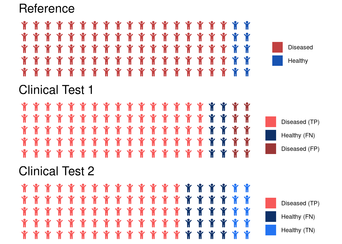
Confusion matrix for the first test
| Prediction/Reference | Diseased | Healthy |
|---|---|---|
| Diseased | TP = 80 | FP = 10 |
| Healthy | FN = 10 | TN = 0 |
Confusion matrix for the second test
| Prediction/Reference | Diseased | Healthy |
|---|---|---|
| Diseased | TP = 70 | FP = 0 |
| Healthy | FN = 20 | TN = 10 |
Comparison of the two tests
Let us compare the performance of the two tests:
| Measure | Test 1 | Test 2 |
|---|---|---|
| Sensitivity (Recall) | 88.9% | 77.7% |
| Specificity | 0% | 100% |
| Precision | 88.9% | 100% |
Considering sensitivity and specificity, we would not select the first test because its balanced accuracy is merely \(\frac{0 + 0.889}{2} = 44.5\%\), while that of the second test is \(\frac{0.777 + 1}{2} = 88.85\%\).
Using precision and recall, however, the first test would have an F1-score of \(2 \cdot \frac{0.889 \cdot 0.889}{0.889 + 0.889} = 0.889\), while the second test has a lower score of \(2 \cdot \frac{0.777 \cdot 1}{0.777 + 1} \approx 0.87\). Thus, we would find the first test to be superior over the second test although its specificity is a 0%. Thus, when using this test, all of the healthy patients would be classified as diseased. This would be a big problem because all of these patients would undergo severe psychological stress and expensive treatment due to the misdiagnosis. If we had used specificity instead, we would have selected the second model, which does not produce any false postives at a competitive sensitivity.
Use of precision when true negatives do not matter
Let us consider an example from information retrieval to illustrate when precision is a useful criterion. Assume that we want to compare two algorithms for document retrieval that both have have an accuracy of 80%.
library(waffle)
colors <- c("#c14141", "#1853b2")
iron(
    waffle(c("Relevant" = 30, "Irrelevant" = 70), rows = 5, use_glyph = "file",
        glyph_size = 5, title = "Reference", colors = ref.colors),
    waffle(c("Relevant (TP)" = 25, "Irrelevant (FN)" = 5, "Relevant (FP)" = 15, "Irrelevant (TN)" = 55),
        rows = 5, use_glyph = "file",
        glyph_size = 5, title = "Retrieval Algorithm 1", colors = c(true.colors[1], false.colors[2], false.colors[1], true.colors[2])),
    waffle(c("Relevant (TP)" = 20, "Irrelevant (FN)" = 10, "Relevant (FP)" = 10, "Irrelevant (TN)" = 60),
        rows = 5, use_glyph = "file",
        glyph_size = 5, title = "Retrieval Algorithm 2", colors = c(true.colors[1], false.colors[2], false.colors[1], true.colors[2]))
)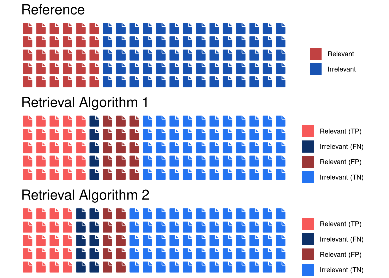
Confusion matrix for the first algorithm
| Prediction/Reference | Relevant | Irrelevant |
|---|---|---|
| Relevant | TP = 25 | FP = 15 |
| Irrelevant | FN = 5 | TN = 55 |
Confusion matrix for the second algorithm
| Prediction/Reference | Relevant | Irrelevant |
|---|---|---|
| Relevant | TP = 20 | FP = 10 |
| Irrelevant | FN = 10 | TN = 60 |
Comparison of the two algorithms
Let us calculate the performance of the two algorithms from the confusion matrix:
| Measure | Algorithm 1 | Algorithm 2 |
|---|---|---|
| Sensitivity (Recall) | 83.3% | 66.7% |
| Specificity | 78.6% | 85.7% |
| Precision | 62.5% | 66.7% |
| Balanced accuracy | 80.95% | 76.2% |
| F1-score | 71.4% | 66.7% |
In this example, both balanced accuracy and the F1-score would lead to prefering the first over the second algorithm. Note that the reported balanced accuracy is decidedly larger than the F1-score. This is because specificity is high for both algorithms due to the large number of discarded observations from the negative class. Since the F1-score does not consider the rate of true negatives, precision and recall are more appropriate than sensitivity and specificity for this task.
Summary
In this post, we have seen that performance measures should be carefully selected. While sensitivity and specificity generally perform well, precision and recall should only be used in circumstances where the true negative rate does not play a role.


Comments
Erbo
02 Dec 18 02:15 UTC
Erbo
02 Dec 18 02:26 UTC
Matthias Döring
02 Dec 18 09:52 UTC
Thanks for your comments Erbo. You’re right about the ordering in the table - the positive class should definitely come first, I just changed this. Regarding the ordering of predicted/reference I’m not sure, I think I have seen both versions, so I will keep it as is. I hope it’s not too confusing ;-) I agree, however, that it would make things much easier if there was really a standard for the format of confusion matrices.
In the second example, the rate rates were indeed off for the second example. It should be fixed now :-) Thanks for having a keen eye!
Fluff
26 Nov 19 15:47 UTC
This is an excellent article! There are very few posts out there comparing specificity vs precision approaches from a “Why” perspective and in such a well thought out way. Thank you!
There is a mistake under “What can go wrong when using precision” You say “Precision is a particularly bad measure when there are few observations that belong to the positive class. Let us assume a clinical data set in which 90% of persons are diseased (positive class) and only 10% are healthy (negative class)”
(You’re firstly saying that precision is a bad measure when the positive class is a minority. You then go on to give an example where 90% of population are in positive class.)